
[Python] 머신러닝 완벽가이드 - 04. 분류[랜덤포레스트,GBM]
Updated:
파이썬 머신러닝 완벽가이드 교재를 토대로 공부한 내용입니다.
실습과정에서 필요에 따라 내용의 누락 및 추가, 수정사항이 있습니다.
기본 세팅
import numpy as np
import pandas as pd

import matplotlib as mpl
import matplotlib.pyplot as plt
import seaborn as sns

import warnings
%matplotlib inline
%config InlineBackend.figure_format = 'retina'

mpl.rc('font', family='NanumGothic') # 폰트 설정
mpl.rc('axes', unicode_minus=False) # 유니코드에서 음수 부호 설정

# 차트 스타일 설정
sns.set(font="NanumGothic", rc={"axes.unicode_minus":False}, style='darkgrid')
plt.rc("figure", figsize=(10,8))

warnings.filterwarnings("ignore")
1. 앙상블 학습 유형
앙상블 학습 유형은 전통적으로 보팅(Voting), 배깅(Bagging), 부스팅(Boosting)의 세 가지로 나눌 수 있으며,
이외에도 스태킹 등 다양한 앙상블 학습 방법이 있다.
보팅(Voting)
- 여러 개의 분류기가 투표를 통해 최종 예측 결과를 결정하는 방식으로, 일반적으로 서로 다른 알고리즘의 분류기를 결합
배깅(Bagging)
-
보팅과 마찬가지로 여러 분류기로 최종 예측 결과를 결정하지만, 동일한 분류기를 데이터 샘플링을 서로 다르게 가져가면서 학습을 수행한다.
-
데이터 샘플링 방식은 부트스트래핑(Bootstrapping)이며 교차 검증과 다르게 데이터의 중복이 허용된다.
-
대표적인 배깅 방식으로 랜덤 포레스트가 있다.
부스팅(Bossting)
-
여러 개의 분류기가 순차적으로 학습을 수행하되, 앞에서 학습한 분류기가 예측이 틀린 데이터에 대해서는
올바르게 예측할 수 있도록 다음 분류기에게는 가중치를 부여하면서 학습과 예측을 진행한다.
-
대표적인 부스팅 방식으로 GBM(Gradient Boosting Machine), XGBoost(eXtra Gradient Boost), LightGBM(Light Gradient Boost)이 있다.
2. 보팅
2.1 하드 보팅
- 하드 보팅은 다수결 원칙과 비슷한 개념으로서 다수의 분류기가 결정한 예측값을 최종 보팅 결과값으로 선정한다.
2.2 소프트 보팅
-
소프트 보팅은 분류기들의 레이블 값 결정 확률을 모두 더하고 평균을 구해 확률이 가장 높은 레이블 값을 최종 보팅 결과값으로 선정한다.
-
일반적으로 소프트 보팅이 예측 성능이 좋아서 더 많이 사용된다.
2.3 breast_cancer 예제
from sklearn.ensemble import VotingClassifier
from sklearn.linear_model import LogisticRegression
from sklearn.neighbors import KNeighborsClassifier
from sklearn.datasets import load_breast_cancer
from sklearn.model_selection import train_test_split
from sklearn.metrics import accuracy_score

# breast_cancer data
cancer = load_breast_cancer()

data_df = pd.DataFrame(cancer.data, columns=cancer.feature_names)
data_df.head()
| mean radius | mean texture | mean perimeter | mean area | mean smoothness | mean compactness | mean concavity | mean concave points | mean symmetry | mean fractal dimension | ... | worst radius | worst texture | worst perimeter | worst area | worst smoothness | worst compactness | worst concavity | worst concave points | worst symmetry | worst fractal dimension | |
|---|---|---|---|---|---|---|---|---|---|---|---|---|---|---|---|---|---|---|---|---|---|
| 0 | 17.99 | 10.38 | 122.80 | 1001.0 | 0.11840 | 0.27760 | 0.3001 | 0.14710 | 0.2419 | 0.07871 | ... | 25.38 | 17.33 | 184.60 | 2019.0 | 0.1622 | 0.6656 | 0.7119 | 0.2654 | 0.4601 | 0.11890 |
| 1 | 20.57 | 17.77 | 132.90 | 1326.0 | 0.08474 | 0.07864 | 0.0869 | 0.07017 | 0.1812 | 0.05667 | ... | 24.99 | 23.41 | 158.80 | 1956.0 | 0.1238 | 0.1866 | 0.2416 | 0.1860 | 0.2750 | 0.08902 |
| 2 | 19.69 | 21.25 | 130.00 | 1203.0 | 0.10960 | 0.15990 | 0.1974 | 0.12790 | 0.2069 | 0.05999 | ... | 23.57 | 25.53 | 152.50 | 1709.0 | 0.1444 | 0.4245 | 0.4504 | 0.2430 | 0.3613 | 0.08758 |
| 3 | 11.42 | 20.38 | 77.58 | 386.1 | 0.14250 | 0.28390 | 0.2414 | 0.10520 | 0.2597 | 0.09744 | ... | 14.91 | 26.50 | 98.87 | 567.7 | 0.2098 | 0.8663 | 0.6869 | 0.2575 | 0.6638 | 0.17300 |
| 4 | 20.29 | 14.34 | 135.10 | 1297.0 | 0.10030 | 0.13280 | 0.1980 | 0.10430 | 0.1809 | 0.05883 | ... | 22.54 | 16.67 | 152.20 | 1575.0 | 0.1374 | 0.2050 | 0.4000 | 0.1625 | 0.2364 | 0.07678 |
5 rows × 30 columns
# 학습/검증 데이터 분리
X_train, X_test, y_train, y_test = train_test_split(cancer.data, cancer.target,
                                                    test_size=0.2, random_state=11)

# 개별 분류기
lr_clf = LogisticRegression()
knn_clf = KNeighborsClassifier(n_neighbors=8)

# 소프트 보팅 기반의 앙상블 모델 분류기
vo_clf = VotingClassifier(estimators = [("LR", lr_clf), ("KNN", knn_clf)], voting = "soft")
-
보팅 분류기
VotingClassifier()의estimators에는 리스트 값으로Classifier객체들을 튜플 형식으로 입력한다. -
voting은 보팅 방식을 설정하며 디폴트 값은 hard이다.
# 개별 분류기 및 보팅 분류기 학습/예측/평가
calssifiers = [vo_clf, lr_clf, knn_clf]

for classifier in calssifiers:
    classifier.fit(X_train, y_train)
    pred = classifier.predict(X_test)
    acc1 = accuracy_score(y_test, pred)

    class_name = classifier.__class__.__name__

    print(f"{class_name} 정확도:{acc1: .4f}")
VotingClassifier 정확도: 0.9737
LogisticRegression 정확도: 0.9386
KNeighborsClassifier 정확도: 0.9561
- 보팅 분류기의 정확도가 가장 높게 나타났는데, 무조건적으로 기반 분류기보다 예측 성능이 향상되는 것은 아니다.
3. 배깅
3.1 랜덤 포레스트
-
랜덤 포레스트는 결정 트리를 기반으로 하는 방식으로서 여러 개의 결정 트리 분류기가 전체 데이터에서 배깅 방식으로 각자의 데이터를 샘플링 한 후
학습을 수행한 뒤 최종적으로 모든 분류기가 보팅을 통해 예측을 결정한다.
-
부트스트래핑 방식으로 데이터를 추출하며, 만약 데이터의 갯수가 100개이고 결정 트리 분류기가 3개이면 데이터 갯수가 100개인 서브셋을 3개 생성한다.
이 때, 각 서브셋에는 개별 데이터가 중복되어 만들어진다.
3.2 사용자 행동 인식 예제
# 피처명 중복 제거
def get_new_feature_name(old_feature_name_df):
    # cumcount()로 피처명별로 중복 존재시 숫자 부여, reset_index()로 Column_Index 생성
    feature_dup = pd.DataFrame(old_feature_name_df.groupby("Column_name").cumcount()).reset_index()

    # features.txt의 Column_Index는 1부터 시작이므로 동일하게 설정
    feature_dup.columns = ["Column_Index", "dup_cnt"]
    feature_dup["Column_Index"] = feature_dup["Column_Index"] + 1

    # Column_Index를 기준으로 Merge 후 중복컬럼명 변경
    temp = pd.merge(old_feature_name_df, feature_dup, on = "Column_Index", how="outer")
    temp["Column_name"] = temp.apply(lambda x: x.Column_name + "_" + str(x.dup_cnt) if x.dup_cnt > 0
                                     else x.Column_name, axis=1)

    return temp

def get_human_dataset():
    # 피처명 불러오기
    feature_name_df = pd.read_csv("./Human_activity/features.txt", sep="\s+", header=None,
                               names = ["Column_Index", "Column_name"])
    # 피처명 중복 수정
    new_feature_name = get_new_feature_name(feature_name_df)

    # 리스트로 변경
    feature_name = new_feature_name["Column_name"].tolist()

    # train, test 피처 데이터(X), 레이블 데이터(y) 로드
    X_train = pd.read_csv("./Human_activity/train/X_train.txt", sep="\s+", names = feature_name)
    X_test = pd.read_csv("./Human_activity/test/X_test.txt", sep="\s+", names = feature_name)

    y_train = pd.read_csv("./Human_activity/train/y_train.txt", sep="\s+", names = ["action"])
    y_test = pd.read_csv("./Human_activity/test/y_test.txt", sep="\s+", names = ["action"])

    return X_train, X_test, y_train, y_test
- 이전 포스팅 에서 정의한 사용자 행동 인식 데이터 불러오기 함수를 사용한다.
from sklearn.ensemble import RandomForestClassifier

X_train, X_test, y_train, y_test = get_human_dataset()

# 랜덤 포레스트 분류기
rf_clf = RandomForestClassifier(random_state=0)
rf_clf.fit(X_train, y_train)
pred = rf_clf.predict(X_test)
acc2 = accuracy_score(y_test, pred)

print(f"랜덤 포레스트 정확도:{acc2: .4f}")
랜덤 포레스트 정확도: 0.9253
- 랜덤 포레스트는 사용자 행동 인식 데이터 셋에 대해 약 92.53%의 정확도를 보여준다.
3.3 랜덤 포레스트 하이퍼 파라미터
랜덤 포레스트의 하이퍼 파라미터는 대부분 결정 트리에서 사용되는 하이퍼 파라미터와 같다.
-
n_estimators: 결정 트리의 갯수를 지정한다. 디폴트는 10개이다. -
max_features: 결정 트리에선 디폴트 값이 전체 피처인 반면, 랜덤 포레스트에선 디폴트로 전체 피처의 “sqrt”만큼 참조한다.
GridSearchCV
from sklearn.model_selection import GridSearchCV

params = {
    "n_estimators": [100],
    "max_depth": [6, 8, 10, 12],
    "min_samples_leaf": [8, 12, 18],
    "min_samples_split": [8, 16, 20]
}

# 랜덤 포레스트 객체 생성 후 GridSearchCV
rf_clf = RandomForestClassifier(random_state=0, n_jobs=-1)
grid_cv = GridSearchCV(rf_clf, param_grid = params, cv=2, n_jobs = -1)

grid_cv.fit(X_train, y_train)

print("최고 예측 정확도:{0:.4f}".format(grid_cv.best_score_))
print("최적 하이퍼 파라미터:\n", grid_cv.best_params_)
최고 예측 정확도:0.9180
최적 하이퍼 파라미터:
 {'max_depth': 10, 'min_samples_leaf': 8, 'min_samples_split': 8, 'n_estimators': 100}
RandomForestClassifier(),GridSearchCV()에서 n_jobs = -1을 추가하면 모든 CPU 코어를 이용해 학습할 수 있다.
best_rt_clf = grid_cv.best_estimator_
rt_pred = best_rt_clf.predict(X_test)
acc = accuracy_score(y_test, rt_pred)

print(f"예측 정확도:{acc: .4f}")
예측 정확도: 0.9196
- 앞서 확인한 최적 하이퍼 파라미터를 적용하였을 때 test 데이터 셋의 예측 정확도는 약 91.96%이다.
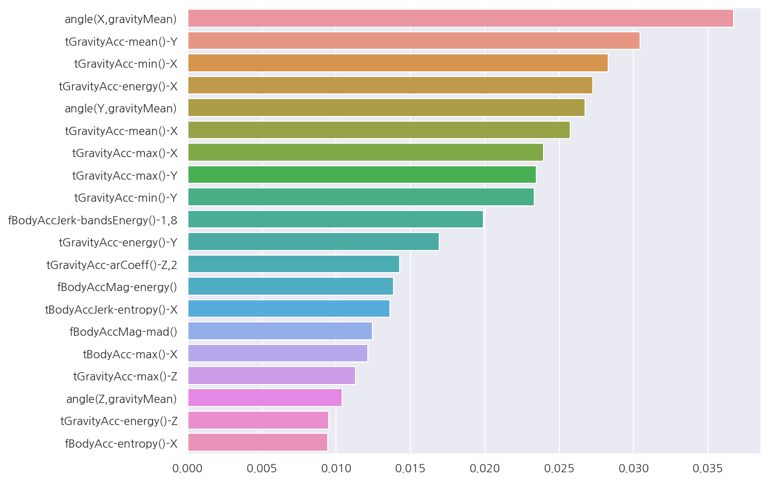
피처별 중요도
# 피처별 중요도 상위 20개
temp = best_rt_clf.feature_importances_
feature_importances_HAR_top20 = pd.Series(temp, index = X_train.columns).sort_values(ascending=False)[:20]

# 시각화
sns.barplot(x = feature_importances_HAR_top20, y = feature_importances_HAR_top20.index)
plt.show()
4. 부스팅
4.1 GBM(Gradient Boosting Machine)
GBM은 여러 개의 weak learner를 순차적으로 학습,예측하면서 잘못 예측한 데이터에 가중치 부여를 통해 오류를 개선해 나가면서 학습하는 방식이다.
가중치의 업데이트 방법은 경사 하강법(Gradient Descent)을 사용한다.
-
경사 하강법(Gradient Descent)
분류의 실제 결과값을 $y$, 피처를 $x_{1}, x_{2}, …, x_{n}$, 피처에 기반한 예측 함수를 $F(x)$ 라고 할 때,
오류식 $h(x) = y - F(x)$을 최소화하는 방향성을 가지고 반복적으로 가중치 값을 업데이트 하는 것이다.
4.2 사용자 행동 인식 예제
from sklearn.ensemble import GradientBoostingClassifier
import time

X_train, X_test, y_train, y_test = get_human_dataset()

# GBM 수행 시간 측정
start_time = time.time()

# GBM
gb_clf = GradientBoostingClassifier(random_state=0)
gb_clf.fit(X_train, y_train)
gb_pred = gb_clf.predict(X_test)
gb_accuray = accuracy_score(y_test,gb_pred)

print(f"GBM 정확도: {gb_accuray:.4f}")
print(f"GBM 수행 시간: {time.time() - start_time:.1f}초")
GBM 정확도: 0.9389
GBM 수행 시간: 1046.9초
4.3 GBM 하이퍼 파라미터
-
loss: 경사 하강법에서 사용할 비용 함수를 지정한다. 특별한 이유가 없다면 디폴트 값 “deviance”를 적용한다. -
learning_rate: GBM이 학습을 진행할 때마다 적용하는 학습률로서 weak learner가 순차적으로 오류 값을 보정해 나가는 데 적용하는 계수0~1 사이의 값을 지정할 수 있고 디폴트는 0.1이다. 값이 작을수록 최소 오류 값을 찾아 예측 성능이 높아질 가능성이 크지만 수행 시간이 오래걸린다. -
n_estimators: weak learner의 갯수로 디폴트 값은 100이다. -
subsample: weak learner가 학습에 사용하는 데이터의 샘플링 비율로 디폴트 값은 1이다.과적합이 염려되는 경우 1보다 작은 값으로 설정한다
GridSearchCV
from sklearn.model_selection import GridSearchCV

params = {"n_estimators": [100, 500], "learning_rate": [0.05, 0.1]}

# GBM 객체 생성 후 GridSearchCV
gb_clf = GradientBoostingClassifier(random_state=0)
grid_cv2 = GridSearchCV(gb_clf, param_grid = params, cv=2, verbose=1)

grid_cv2.fit(X_train, y_train)

print("최고 예측 정확도:{0:.4f}".format(grid_cv2.best_score_))
print("최적 하이퍼 파라미터:\n", grid_cv2.best_params_)
Fitting 2 folds for each of 4 candidates, totalling 8 fits


[Parallel(n_jobs=1)]: Using backend SequentialBackend with 1 concurrent workers.
[Parallel(n_jobs=1)]: Done   8 out of   8 | elapsed: 217.5min finished


최고 예측 정확도:0.9011
최적 하이퍼 파라미터:
 {'learning_rate': 0.1, 'n_estimators': 500}
-
GBM으로 간단히 최적 하이퍼 파라미터와 최고 예측 정확도를 구하였다.
-
소요시간이 굉장히 오래 걸리는 것을 확인 할 수 있다.
best_gb_clf = grid_cv2.best_estimator_
gb_pred = best_gb_clf.predict(X_test)
acc = accuracy_score(y_test, gb_pred)

print(f"예측 정확도:{acc: .4f}")
예측 정확도: 0.9420
- 앞서 확인한 최적 하이퍼 파라미터를 적용하였을 때 test 데이터 셋의 예측 정확도는 약 94.20%이다.
Leave a comment