[Python] 머신러닝 완벽가이드 - 04. 분류[결정트리]

Updated: June 17, 2021

파이썬 머신러닝 완벽가이드 교재를 토대로 공부한 내용입니다.

실습과정에서 필요에 따라 내용의 누락 및 추가, 수정사항이 있습니다.

기본 세팅

import numpy as np
import pandas as pd

import matplotlib as mpl
import matplotlib.pyplot as plt
import seaborn as sns

import warnings

%matplotlib inline
%config InlineBackend.figure_format = 'retina'

mpl.rc('font', family='NanumGothic') # 폰트 설정
mpl.rc('axes', unicode_minus=False) # 유니코드에서 음수 부호 설정

# 차트 스타일 설정
sns.set(font="NanumGothic", rc={"axes.unicode_minus":False}, style='darkgrid')
plt.rc("figure", figsize=(10,8))

warnings.filterwarnings("ignore")

1. 결정 트리

결정 트리는 데이터에 있는 규칙을 학습을 통해 자동으로 찾아내 트리 기반의 분류 규칙을 만드는 것으로 스무고개와 비슷한 개념이다.

결정 트리는 다음과 같은 노드로 구성되어 있다.

루트 노드(Root Node): 초기 지점으로 첫 번째 분류 규칙 노드
브랜치 노드(Branch Node): 자식 노드를 가지는 중간 규칙 노드로서 브랜치 노드, 리프 노드로 분리 될 수 있다.
리프 노드(Leaf Node): 더 이상 자식 노드가 없는 노드로서 최종 클래스 값이 결정되는 노드

여기서 규칙은 정보 균일도가 높은 데이터 셋을 먼저 선택할 수 있도록 규칙 조건을 만들며, 정보 균일도를 측정하는 대표적인 방법은 다음과 같다.

엔트로피 지수: 주어진 데이터 집합의 혼잡도를 의미하며 서로 다른 값이 섞여 있으면 값이 커지고, 같은 값이 섞여 있으면 값이 낮아진다.
지니 계수: 불평등 지수로 값이 0일때 가장 평등하고 1에 가까워질수록 불평등 해진다.

모든 데이터가 같은 값을 가지면 엔트로피 지수는 0이 된다.

머신러닝에선 각 영역의 지니 계수가 낮은 속성을 기준으로 분할한다.

1.1 결정 트리 모델의 시각화

from sklearn.tree import DecisionTreeClassifier
from sklearn.datasets import load_iris
from sklearn.model_selection import train_test_split

# iris data
iris_data = load_iris()
X_train, X_test, y_train, y_test = train_test_split(iris_data.data, iris_data.target, test_size=0.2, random_state=11)

# DecisionTreeClassifier 객체 생성, 학습
dt_clf = DecisionTreeClassifier(random_state=156)
dt_clf.fit(X_train, y_train)

DecisionTreeClassifier(random_state=156)

from sklearn.tree import export_graphviz

export_graphviz(dt_clf, out_file="tree.dot", 
                class_names= iris_data.target_names, 
                feature_names = iris_data.feature_names, 
                impurity = True,
                filled= True)

export_graphviz()에 학습이 완료된 estimator(), output 파일 명, 결정 클래스 명칭 등을 입력한다.

import graphviz

with open("tree.dot") as f:
    dot_graph = f.read()

graphviz.Source(dot_graph)

svg

Root Node

첫 번째 루트 노드에는 train 데이터 샘플 120개 전체가 있고 지니 계수 및 현재 value 구성을 확인 할 수 있다.
Petal Length <= 2.45 규칙으로 자식 노드를 생성하며 class는 하위 노드를 가질 경우 setosa가 41개로 가장 많다는 의미이다.

Leaf Node

두 번째 리프 노드는 Petal Length <= 2.45가 True인 경우로 모든 클래스가 setosa로 결정 되어 지니 계수가 0이다.

Branch Node

세 번째 브랜치 노드는 Petal Length <= 2.45가 False인 경우로 지니 계수가 0.5로 높으므로 다음 자식 브랜치 노드로 분기할 규칙이 필요하다.
Petal Width <= 1.55 규칙으로 자식 노드를 생성한다.

Else

각 노드의 색깔은 붓꽃 데이터의 레이블 값을 의미하며 색깔이 짙어질수록 지니 계수가 낮고 해당 레이블에 속하는 샘플 데이터가 많다는 의미이다.
네 번째 브랜치 노드를 보면 virginica가 단 1개이고, versicolr가 37개인데 이를 구분하기 위해 또 다시 자식 노드를 생성한다.
결정 트리는 규칙 생성 로직을 제어하지 않으면 완벽하게 클래스를 구분하기 위해 노드를 계속 생성하며 이는 과적합 문제로 이어진다.

1.2 결정 트리 모델의 하이퍼 파라미터

Iris Tree 함수

from sklearn.tree import export_graphviz
import graphviz

def iris_tree_hyper(max_dep = None, min_ss = 2, min_sl = 1):
    # DecisionTreeClassifier 객체 생성, 학습
    dt_clf = DecisionTreeClassifier(random_state = 156, 
                                    max_depth = max_dep, 
                                    min_samples_split = min_ss, 
                                    min_samples_leaf = min_sl
                                    )
    dt_clf.fit(X_train, y_train)

    # Graphviz 출력 파일 생성 및 리드
    export_graphviz(dt_clf, out_file="tree.dot", 
                    class_names= iris_data.target_names, 
                    feature_names = iris_data.feature_names, 
                    impurity = True,
                    filled= True)

    with open("tree.dot") as f:
        dot_graph = f.read()

    return graphviz.Source(dot_graph)

iris_tree_hyper()

svg

하이퍼 파라미터 옵션을 디폴트로 적용하여 앞서 출력한 결과와 동일하다.

1.2.1 깊이 조건

iris_tree_hyper(max_dep=2)

svg

하이퍼 파라미터 max_depth를 2로 제한하여 더 간단한 결정 트리를 생성하였다.

1.2.2 최소 분할 샘플 조건

iris_tree_hyper(min_ss=4)

svg

하이퍼 파라미터 min_samples_split을 4로 제한하여 각 노드에서 샘플이 4개 이상인 경우만 분기하도록 설정하였다.

1.2.3 최소 리프 샘플 조건

iris_tree_hyper(min_sl=10)

svg

하이퍼 파라미터 min_samples_leaf를 10으로 제한하여 각 노드에서 샘플이 10개 이상인 경우 리프 노드가 될 수 있다.

1.3 피처별 중요도

# 학습된 DecisionTreeClassifier 객체의 feature_importances_ 속성
feature_imp = dt_clf.feature_importances_

# 피처별 중요도
print("# 피처별 중요도")
for name, value in zip(iris_data.feature_names, feature_imp):
    print(f"{name}: {value:.4f}")
    
# 시각화
sns.barplot(x = feature_imp, y = iris_data.feature_names)
plt.show()

# 피처별 중요도
sepal length (cm): 0.0250
sepal width (cm): 0.0000
petal length (cm): 0.5549
petal width (cm): 0.4201

png

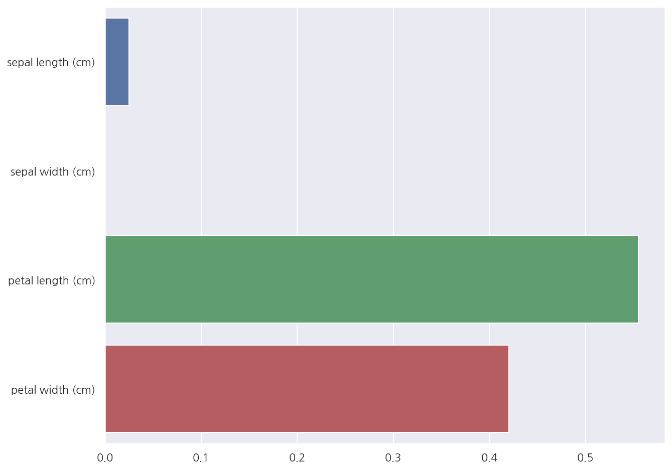
Petal length가 피처 중요도가 가장 높음을 알 수 있다.

1.4 결정 트리 과적합

1.4.1 분류용 가상 데이터

make_classification

분류용 가상 데이터를 생성하는 make_classification()의 인수는 다음과 같다.

n_samples : 표본 데이터의 수, 디폴트 100
n_features : 독립 변수의 수, 디폴트 20
n_informative : 독립 변수 중 종속 변수와 상관 관계가 있는 성분의 수, 디폴트 2
n_redundant : 독립 변수 중 다른 독립 변수의 선형 조합으로 나타나는 성분의 수, 디폴트 2
n_repeated : 독립 변수 중 단순 중복된 성분의 수, 디폴트 0
n_classes : 종속 변수의 클래스 수, 디폴트 2
n_clusters_per_class : 클래스 당 클러스터의 수, 디폴트 2
weights : 각 클래스에 할당된 표본 수
random_state : 난수 발생 시드

출력은 다음과 같다.

X : [n_samples, n_features] 크기의 배열
y : [n_samples] 크기의 배열

출처: 데이터 사이언스 스쿨: https://datascienceschool.net/intro.html

가상 데이터 생성

from sklearn.datasets import make_classification

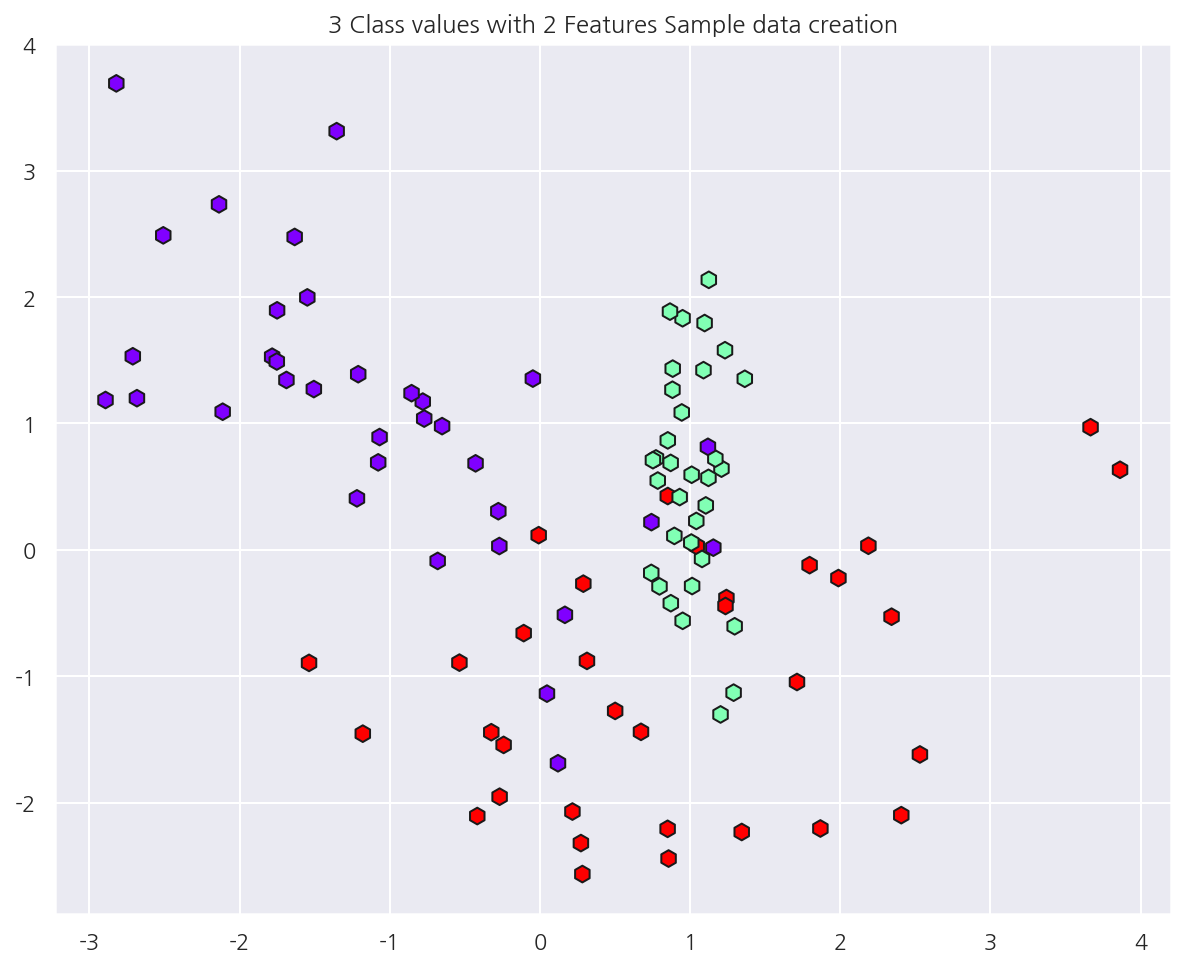
# 피처 2개, 클래스 3개인 가상 데이터
X_features, y_labels = make_classification(n_features = 2, n_redundant = 0, n_informative = 2, 
                                           n_classes = 3, n_clusters_per_class = 1, random_state = 0)

x1 = X_features[:,0]
x2 = X_features[:,1]

# 시각화
plt.scatter(x1 ,x2 , marker="h", c=y_labels, cmap='rainbow', s=70, edgecolor ="k")

plt.title("3 Class values with 2 Features Sample data creation")
plt.show()

png

1.4.2 과적합 문제 시각화

결정 트리 경계 시각화 함수

def visualize_boundary(model, X, y):
    fig, ax = plt.subplots()
    
    # 학습 데이터 scatter plot으로 나타내기
    ax.scatter(X[:, 0], X[:, 1], c=y, s=25, cmap='rainbow', edgecolor='k',
               clim=(y.min(), y.max()), zorder=3)
    ax.axis('tight')
    ax.axis('off')
    xlim_start , xlim_end = ax.get_xlim()
    ylim_start , ylim_end = ax.get_ylim()
    
    # model 학습 
    model.fit(X, y)
    
    # meshgrid 형태인 모든 좌표값으로 예측 수행. 
    xx, yy = np.meshgrid(np.linspace(xlim_start,xlim_end, num=200),np.linspace(ylim_start,ylim_end, num=200))
    Z = model.predict(np.c_[xx.ravel(), yy.ravel()]).reshape(xx.shape)
    
    # contourf() 를 이용하여 class boundary 를 visualization 수행. 
    n_classes = len(np.unique(y))
    contours = ax.contourf(xx, yy, Z, alpha=0.3,
                           levels=np.arange(n_classes + 1) - 0.5,
                           cmap='rainbow', clim=(y.min(), y.max()),
                           zorder=1)

책의 부록으로 제공되는 소스 코드를 사용하였다.

트리 생성 제약이 없는 경우

from sklearn.tree import DecisionTreeClassifier

dt_clf = DecisionTreeClassifier(random_state = 10)
dt_clf.fit(X_features, y_labels)

visualize_boundary(dt_clf, X_features, y_labels)

png

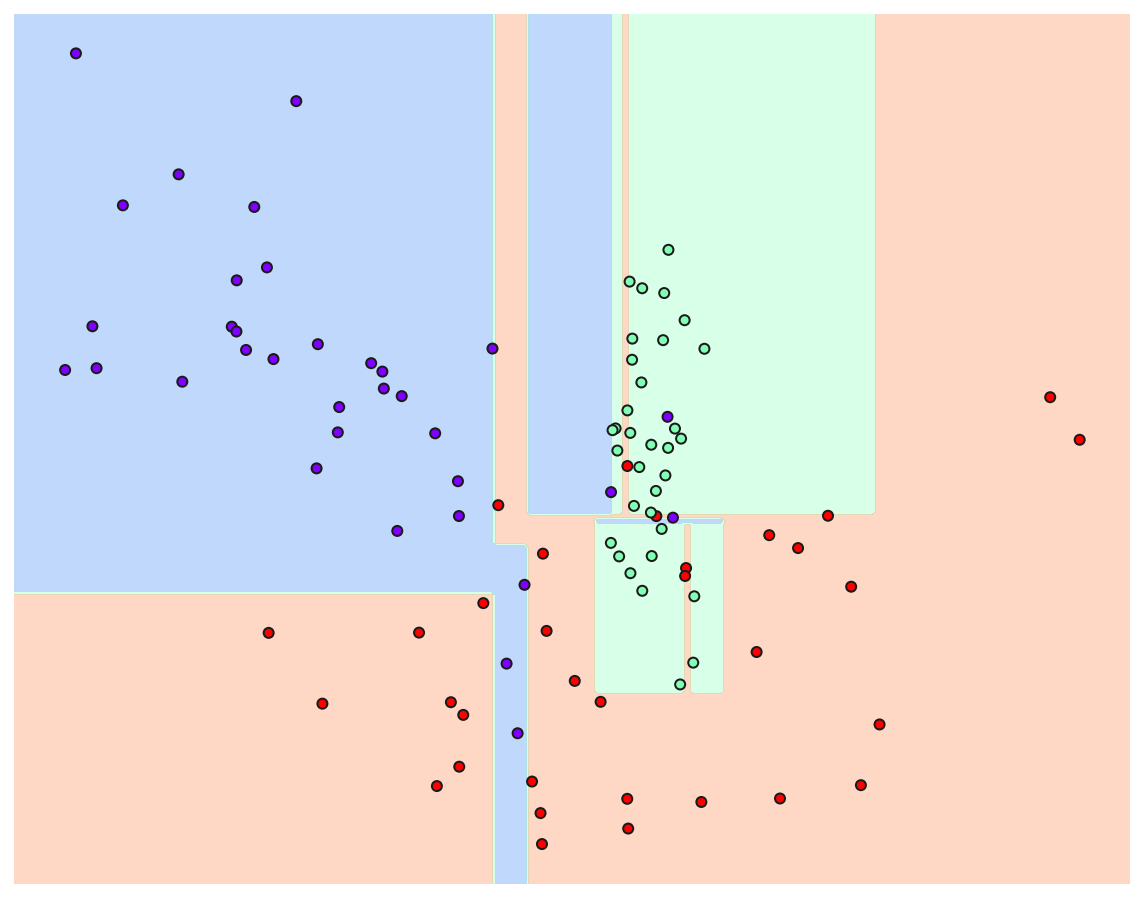
이상치 데이터까지 분류하기 위해 분기가 자주 일어나면서 결정 기준 경계가 많아진 것을 확인 할 수 있다.
즉, 주어진 데이터에 맞추어 과적합 된 상태이며 이는 새로운 데이터에 대해서는 예측 정확도가 떨어질 수 밖에 없다.

트리 생성 제약이 있는 경우

from sklearn.tree import DecisionTreeClassifier

dt_clf = DecisionTreeClassifier(random_state = 10, min_samples_leaf=6)
dt_clf.fit(X_features, y_labels)

visualize_boundary(dt_clf, X_features, y_labels)

png

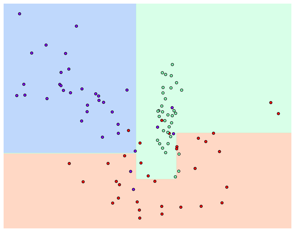
mean_samples_leaf를 6으로 설정하여 제약이 없는 경우에 비해 일반화된 분류 규칙에 따라 분류함을 알 수 있다.

1.5 결정 트리 실습

1.5.1 데이터 설명

실습 데이터는 UCI 머신러닝 리포지토리에서 제공하는 사용자 행동 인식(Human Activity Recognition) 데이터를 사용한다.

해당 데이터는 30명에게 스마트폰 센서를 장착한 뒤 사람의 동작과 관련된 여러 가지 피처를 수집한 데이터이다.

1.5.2 데이터 불러오기

피처 정보 불러오기

feature_name_df = pd.read_csv("./Human_activity/features.txt", sep="\s+", header=None,
                               names = ["Column_Index", "Column_name"])

# feature_name_df.shape[0]
feature_name_df.head()

	Column_Index	Column_name
0	1	tBodyAcc-mean()-X
1	2	tBodyAcc-mean()-Y
2	3	tBodyAcc-mean()-Z
3	4	tBodyAcc-std()-X
4	5	tBodyAcc-std()-Y

features.txt에는 561개의 피처 Index와 피처명이 저장되어 있다.
주의할 점으로 features.txt에는 중복된 피처명이 존재하며 이를 이용하여 데이터를 로드시 오류가 발생한다.

피처명 중복 확인

temp = feature_name_df.groupby("Column_name").count().sort_values(by="Column_Index", ascending=False)
feature_dup = temp[temp["Column_Index"] > 1]

print("중복된 피처 수:", feature_dup.count()[0])
feature_dup.head()

중복된 피처 수: 42

	Column_Index
Column_name
fBodyAccJerk-bandsEnergy()-9,16	3
fBodyAccJerk-bandsEnergy()-1,16	3
fBodyGyro-bandsEnergy()-1,8	3
fBodyGyro-bandsEnergy()-17,24	3
fBodyGyro-bandsEnergy()-17,32	3

피처명 중복 제거

def get_new_feature_name(old_feature_name_df):
    # cumcount()로 피처명별로 중복 존재시 숫자 부여, reset_index()로 Column_Index 생성
    feature_dup = pd.DataFrame(old_feature_name_df.groupby("Column_name").cumcount()).reset_index()
    
    # features.txt의 Column_Index는 1부터 시작이므로 동일하게 설정
    feature_dup.columns = ["Column_Index", "dup_cnt"]
    feature_dup["Column_Index"] = feature_dup["Column_Index"] + 1
    
    # Column_Index를 기준으로 Merge 후 중복컬럼명 변경
    temp = pd.merge(old_feature_name_df, feature_dup, on = "Column_Index", how="outer")
    temp["Column_name"] = temp.apply(lambda x: x.Column_name + "_" + str(x.dup_cnt) if x.dup_cnt > 0 
                                     else x.Column_name, axis=1)
    
    return temp

만약 x라는 컬럼명이 3개 있다면 x, x_1, x_2로 변경하는 함수 생성

check = get_new_feature_name(feature_name_df)
check[check.dup_cnt>0].tail(3)

	Column_Index	Column_name	dup_cnt
499	500	fBodyGyro-bandsEnergy()-49,64_2	2
500	501	fBodyGyro-bandsEnergy()-1,24_2	2
501	502	fBodyGyro-bandsEnergy()-25,48_2	2

컬럼명은 잘 변경되었으며, 유의할 점은 dup_cnt값이 2라는 건 fetures.txt에 해당 피처는 총 3(2+1)개 존재한다는 것이다.

데이터 불러오기 함수

def get_human_dataset():
    # 피처명 불러오기
    feature_name_df = pd.read_csv("./Human_activity/features.txt", sep="\s+", header=None,
                               names = ["Column_Index", "Column_name"])
    # 피처명 중복 수정
    new_feature_name = get_new_feature_name(feature_name_df)
    
    # 리스트로 변경
    feature_name = new_feature_name["Column_name"].tolist()
    
    # train, test 피처 데이터(X), 레이블 데이터(y) 로드
    X_train = pd.read_csv("./Human_activity/train/X_train.txt", sep="\s+", names = feature_name)
    X_test = pd.read_csv("./Human_activity/test/X_test.txt", sep="\s+", names = feature_name)
    
    y_train = pd.read_csv("./Human_activity/train/y_train.txt", sep="\s+", names = ["action"])
    y_test = pd.read_csv("./Human_activity/test/y_test.txt", sep="\s+", names = ["action"])
    
    return X_train, X_test, y_train, y_test

데이터 불러오기

X_train, X_test, y_train, y_test = get_human_dataset()

X_train.info()

<class 'pandas.core.frame.DataFrame'>
RangeIndex: 7352 entries, 0 to 7351
Columns: 561 entries, tBodyAcc-mean()-X to angle(Z,gravityMean)
dtypes: float64(561)
memory usage: 31.5 MB

train 데이터는 7352개의 레코드와 561개의 피처로 이루어져 있으며 모든 피처가 float 형태이므로 카테코리 인코딩 작업은 필요없다.

plt.figure(figsize=(10,5))

frequency = y_train['action'].value_counts()

label = []
for key, value in frequency.to_dict().items():
    label.append(f"{key}: {value}개")

plt.pie(frequency,
    startangle = 180,
    counterclock = False,
    explode = [0.03] * len(label),
    autopct = '%1.1f%%',
    labels = label,
    colors = sns.color_palette('pastel', len(label)),
    wedgeprops = dict(width=0.7)
  )


plt.axis('equal')
plt.show()

png

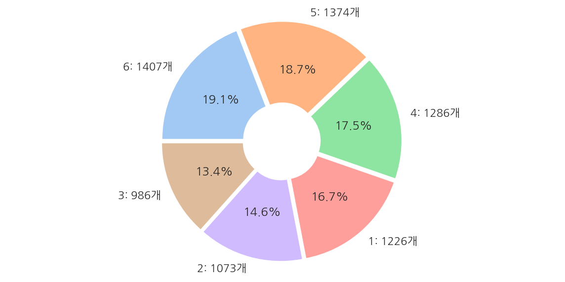
레이블 값은 6개의 클래스로 구성되어 있고 비교적 고르게 분포되어 있다.

1.5.3 성능 평가

1.5.3.1 하이퍼 파라미터 디폴트 성능 평가

from sklearn.tree import DecisionTreeClassifier
from sklearn.metrics import accuracy_score

# 하이퍼 파라미터는 디폴트 값
dt_clf = DecisionTreeClassifier(random_state = 1017)

dt_clf.fit(X_train, y_train)
pred = dt_clf.predict(X_test)
accuracy = accuracy_score(y_test, pred)

print(f"결정 트리 예측 정확도: {accuracy:.4f}")
print(f"\nDecisionTreeClassifier 기본 하이퍼 파라미터:\n{dt_clf.get_params()}")

결정 트리 예측 정확도: 0.8527

DecisionTreeClassifier 기본 하이퍼 파라미터:
{'ccp_alpha': 0.0, 'class_weight': None, 'criterion': 'gini', 'max_depth': None, 'max_features': None, 'max_leaf_nodes': None, 'min_impurity_decrease': 0.0, 'min_impurity_split': None, 'min_samples_leaf': 1, 'min_samples_split': 2, 'min_weight_fraction_leaf': 0.0, 'presort': 'deprecated', 'random_state': 1017, 'splitter': 'best'}

약 85.27%의 정확도를 나타내고 있다.

1.5.3.2 하이퍼 파라미터별 성능 평가

max_depth_lst = [6, 8, 10, 12, 16, 18, 20, 24]

# 하이퍼 파라미터별 예측 정확도
for depth in max_depth_lst:
    dt_clf = DecisionTreeClassifier(random_state = 1017, max_depth = depth)

    dt_clf.fit(X_train, y_train)
    pred = dt_clf.predict(X_test)
    accuracy = accuracy_score(y_test, pred)

    print(f"하이퍼 파라미터 max_depth = {depth}, 결정 트리 예측 정확도: {accuracy:.4f}")

하이퍼 파라미터 max_depth = 6, 결정 트리 예측 정확도: 0.8554
하이퍼 파라미터 max_depth = 8, 결정 트리 예측 정확도: 0.8704
하이퍼 파라미터 max_depth = 10, 결정 트리 예측 정확도: 0.8649
하이퍼 파라미터 max_depth = 12, 결정 트리 예측 정확도: 0.8653
하이퍼 파라미터 max_depth = 16, 결정 트리 예측 정확도: 0.8565
하이퍼 파라미터 max_depth = 18, 결정 트리 예측 정확도: 0.8527
하이퍼 파라미터 max_depth = 20, 결정 트리 예측 정확도: 0.8527
하이퍼 파라미터 max_depth = 24, 결정 트리 예측 정확도: 0.8527

max_depth가 8일때 예측 정확도가 87.04%로 가장 높았고 이후 감소하는 형태이다.

1.5.3.3 GridSearchCV 성능 평가

깊이 조건

from sklearn.model_selection import GridSearchCV

# 하이퍼 파라미터
params = {"max_depth": [6, 8, 10, 12, 16, 18, 20, 24]}

dt_clf = DecisionTreeClassifier(random_state = 1017)

# GridSearchCV
# verbose는 반복시 마다 수행 결과 메시지를 출력한다.
grid_cv = GridSearchCV(dt_clf, param_grid=params, scoring="accuracy", cv=5, verbose=1)
grid_cv.fit(X_train, y_train)

print("GridSearchCV 최적 하이퍼 파라미터:", grid_cv.best_params_)
print("GridSearchCV 최고 평균 정확도:", grid_cv.best_score_.round(4))

Fitting 5 folds for each of 8 candidates, totalling 40 fits

[Parallel(n_jobs=1)]: Using backend SequentialBackend with 1 concurrent workers.
[Parallel(n_jobs=1)]: Done  40 out of  40 | elapsed:  1.6min finished

GridSearchCV 최적 하이퍼 파라미터: {'max_depth': 10}
GridSearchCV 최고 평균 정확도: 0.8554

max_depth가 10일때 5개의 폴드의 평균 정확도가 85.54%로 가장 높았다.

cv_results_df = pd.DataFrame(grid_cv.cv_results_)
cv_results_df[["param_max_depth", "mean_test_score"]]

	param_max_depth	mean_test_score
0	6	0.847255
1	8	0.853518
2	10	0.855427
3	12	0.848217
4	16	0.845767
5	18	0.846992
6	20	0.849031
7	24	0.849847

max_depth가 10을 넘어서면 평균 정확도가 떨어진 것을 확인할 수 있다.
깊이를 너무 증가시키면 train 데이터는 올바르게 예측하겠지만 test 데이터는 과적합으로 인해 잘 예측하지 못한다.
앞서 폴드 없이 하이퍼 파라미터를 변경하면서 train 데이터로 학습 후 test 데이터의 예측 정확도를 구한 것과 달리

현재 GridSearchCV에선 test 데이터는 사용하지 않고 train 데이터를 3개의 폴드로 나눠 그 안에서 test 데이터를 설정하기에 정확도 값에는 차이가 있다.

깊이 조건, 최소 분할 샘플 조건

# 하이퍼 파라미터
params = {
    "max_depth": [8, 12, 16, 20], 
    "min_samples_split": [16, 24]
}

dt_clf = DecisionTreeClassifier(random_state = 1017)

# GridSearchCV
# verbose는 반복시 마다 수행 결과 메시지를 출력한다.
grid_cv = GridSearchCV(dt_clf, param_grid=params, scoring="accuracy", cv=5, verbose=1)
grid_cv.fit(X_train, y_train)

print("GridSearchCV 최적 하이퍼 파라미터:", grid_cv.best_params_)
print("GridSearchCV 최고 평균 정확도:", grid_cv.best_score_.round(4))

Fitting 5 folds for each of 8 candidates, totalling 40 fits

[Parallel(n_jobs=1)]: Using backend SequentialBackend with 1 concurrent workers.
[Parallel(n_jobs=1)]: Done  40 out of  40 | elapsed:  1.7min finished

GridSearchCV 최적 하이퍼 파라미터: {'max_depth': 8, 'min_samples_split': 16}
GridSearchCV 최고 평균 정확도: 0.8565

max_depth와 min_samples_split 조건을 주었을 때 각각 8, 16이 최적 하이퍼 파라미터로 확인된다.
해당 최적 하이퍼 파라미터로 test 데이터에 대해 예측 정확도를 확인한다.

# 최적 하이퍼 파라미터로 예측
best_dt_clf = grid_cv.best_estimator_
pred1 = best_dt_clf.predict(X_test)
accuracy = accuracy_score(y_test, pred1)

print(f"결정 트리 예측 정확도: {accuracy:.4f}")

결정 트리 예측 정확도: 0.8714

최적 하이퍼 파라미터로 test 데이터에 대한 예측 정확도를 구했을 때 약 87.17%로

처음 하이퍼 파라미터를 디폴트 값으로 하였을 때 85.27%보다 상승된 것을 확인 할 수 있다.

1.5.4 피처별 중요도

# 피처별 중요도 상위 20개
feature_importances_HAR = best_dt_clf.feature_importances_
feature_importances_HAR = pd.Series(feature_importances_HAR, index = X_train.columns).sort_values(ascending=False)
feature_importances_HAR_top20 = feature_importances_HAR[:20]

# 시각화
sns.barplot(x = feature_importances_HAR_top20, y = feature_importances_HAR_top20.index)
plt.show()

png

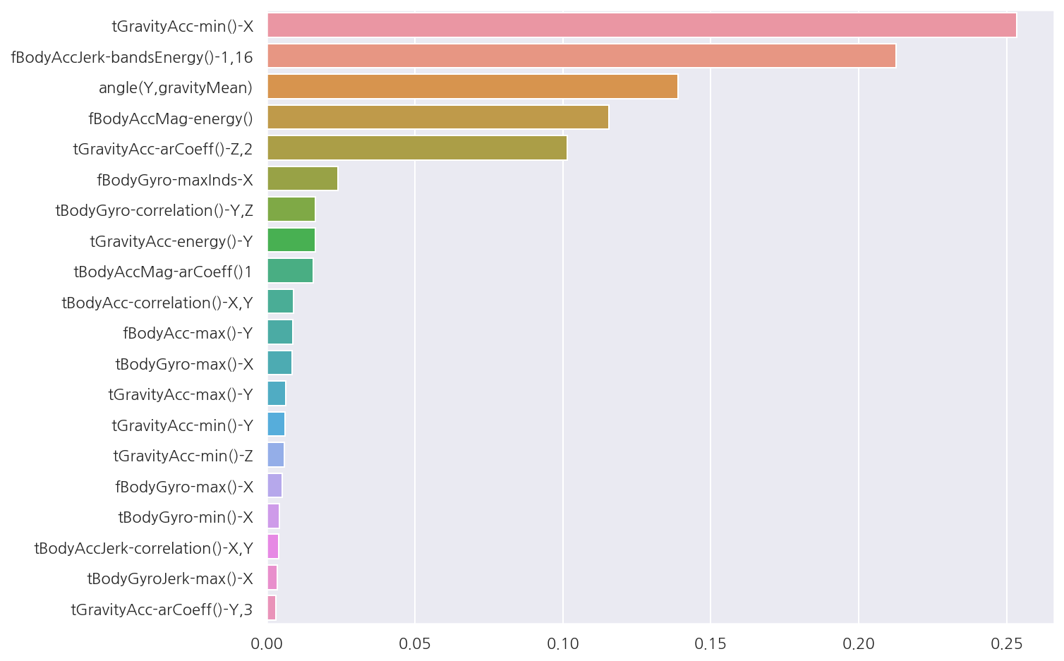
중요도 수치 상위 20개를 확인 하였을 때 특히 상위 5개의 피처가 중요도가 높은 것이 확인된다.

Share on

Twitter Facebook LinkedIn

Romg2