[Python] 머신러닝 완벽가이드 - 06. 차원축소[PCA]

Updated: June 17, 2021

파이썬 머신러닝 완벽가이드 교재를 토대로 공부한 내용입니다.

실습과정에서 필요에 따라 내용의 누락 및 추가, 수정사항이 있습니다.

기본 세팅

import numpy as np
import pandas as pd

import matplotlib as mpl
import matplotlib.pyplot as plt
import seaborn as sns

import warnings

%matplotlib inline
%config InlineBackend.figure_format = 'retina'

mpl.rc('font', family='NanumGothic') # 폰트 설정
mpl.rc('axes', unicode_minus=False) # 유니코드에서 음수 부호 설정

# 차트 스타일 설정
sns.set(font="NanumGothic", rc={"axes.unicode_minus":False}, style='darkgrid')
plt.rc("figure", figsize=(10,8))

warnings.filterwarnings("ignore")

2. PCA(Principal Component Analysis)

PCA

PCA는 가장 대표적인 차원 축소 기법중 하나이다.

여러 변수간에 존재하는 상관관계를 이용해 이를 대표하는 주성분(Principal Component)를 추출해 차원을 축소한다.

PCA는 가장 높은 분산을 가지는 데이터의 축을 찾아 이 축으로 차원을 축소하는데 이것이 PCA의 주성분이 된다.

선형대수에서의 PCA

PCA를 선형대수로 해석하면 입력 데이터의 공분산 행렬을 고유값 분해 후 구한 고유벡터에 입력 데이터를 선형 변환하는 것이다.

고유벡터는 PCA의 주성분 벡터로서 입력 데이터의 분산이 큰 방향을 나타낸다.
고유값은 고유벡터의 크기를 나타내며 동시에 입력 데이터의 분산을 나타낸다.

수식으로 나타내면 다음과 같다.

\[C = \begin{bmatrix} e_{1} & \cdots & e_{n} \end{bmatrix} \begin{bmatrix} \lambda_{1} & \cdots & 0 \\ \vdots & \cdots & \cdots \\ 0 & \cdots & \lambda_{n} \\ \end{bmatrix} \begin{bmatrix} {e_{1}}^{t} \\ \vdots \\ {e_{n}}^{t} \\ \end{bmatrix}\]

공분산 행렬 $C$는 고유벡터 직교행렬 x 고유값 정방행렬 x 고유벡터 직교행렬의 전치행렬로 분해
$e_{i}$, $\lambda_{i}$는 각각 $i$번째 고유벡터, 해당 고유벡터의 크기를 의미한다.
$e_{1}$은 가장 분산이 큰 방향을 가진 고유벡터, $e_{2}$는 $e_{1}$에 수직이면서 다음으로 분산이 큰 방향을 가진 고유벡터

PCA 수행과정

입력 데이터 세트의 공분산 행렬을 생성한다.
공분산 행렬의 고유벡터와 고유값을 계산한다.
고유값이 가장 큰 순으로 K개(PCA의 변환 차수)만큼 고유벡터를 추출한다.
고유값이 가장 큰 순으로 추출된 고유벡터를 이용해 새롭게 입력 데이터를 변환한다.

2.1 IRIS 데이터

from sklearn.datasets import load_iris

iris = load_iris()

columns = ['sepal_length','sepal_width','petal_length','petal_width']
iris_df = pd.DataFrame(data = iris.data, columns = columns)
iris_df["target"] = iris.target

iris_df.head()

	sepal_length	sepal_width	petal_length	petal_width
0	5.1	3.5	1.4	0.2
1	4.9	3.0	1.4	0.2
2	4.7	3.2	1.3	0.2
3	4.6	3.1	1.5	0.2
4	5.0	3.6	1.4	0.2

markers = ["^", "s", "o"]

# 0:setosa, 1:versicolor, 2:virginica
for i, marker in enumerate(markers):
    x_axis_data = iris_df[iris_df['target']==i]['sepal_length']
    y_axis_data = iris_df[iris_df['target']==i]['sepal_width']
    plt.scatter(x_axis_data, y_axis_data, marker=marker, label=iris.target_names[i])

plt.legend()
plt.xlabel('sepal length')
plt.ylabel('sepal width')
plt.show()

png

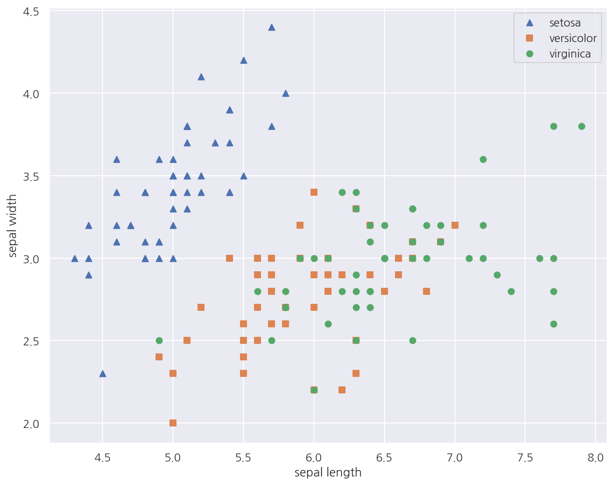
일부 피처에 대해 붓꽃 종류를 시각화 하였다.
setosa의 경우 sepal width가 3이상, sepal length가 6이하인 곳에 대부분 분포되어 있다.
versicolor, virginica는 sepal width, sepal length만으로는 분류하기 어려워 보인다.

from sklearn.preprocessing import StandardScaler

iris_f_scaled = StandardScaler().fit_transform(iris_df.iloc[:,:-1])

PCA는 여러 피처 값을 연산하기에 스케일에 영향을 받으므로 PCA 적용 전에 피처 스케일링 작업이 필요하다.
여기선 StandardScaler()로 표준 정규 분포로 변환하였다.

from sklearn.decomposition import PCA

# 변환할 차원 수 입력
pca = PCA(n_components = 2)

# 스케일 데이터 -> PCA 변환 데이터
pca.fit(iris_f_scaled)
iris_pca = pca.transform(iris_f_scaled)

print(f"스케일 데이터 shape: {iris_f_scaled.shape}")
print(f"PCA 데이터 shape: {iris_pca.shape}")

스케일 데이터 shape: (150, 4)
PCA 데이터 shape: (150, 2)

PCA를 이용해 기존 4차원(4개 피처)에서 2차원으로 변환 하였다.

# PCA 데이터 프레임 생성
pca_columns=['pca_component_1','pca_component_2']

iris_df_pca = pd.DataFrame(iris_pca, columns = pca_columns)
iris_df_pca['target'] = iris.target

iris_df_pca.head(3)

	pca_component_1	pca_component_2
0	-2.264703	0.480027
1	-2.080961	-0.674134
2	-2.364229	-0.341908

markers = ["^", "s", "o"]

# 0:setosa, 1:versicolor, 2:virginica
for i, marker in enumerate(markers):
    x_axis_data = iris_df_pca[iris_df_pca['target']==i]['pca_component_1']
    y_axis_data = iris_df_pca[iris_df_pca['target']==i]['pca_component_2']
    plt.scatter(x_axis_data, y_axis_data, marker=marker,label=iris.target_names[i])

plt.legend()
plt.xlabel('pca_component_1')
plt.ylabel('pca_component_2')
plt.show()

png

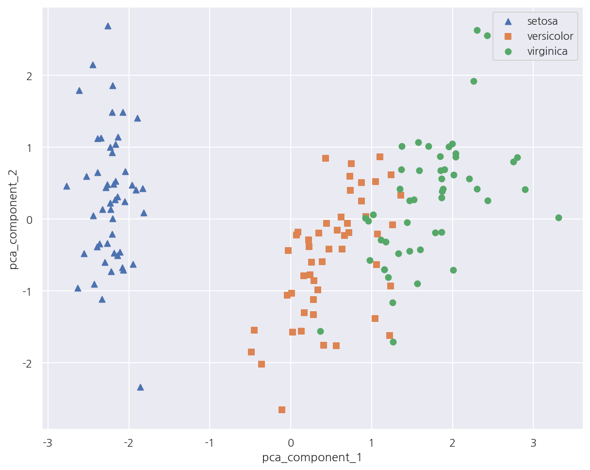
PCA 변환 후 2개의 속성(피처)로 붓꽃 종류를 시각화 하였다.
setosa의 경우 pca_component_1 축을 기반으로 명확하게 구분된다.
versicolor, virginica는 pca_component_1 축을 기반으로 일부 겹치긴 하지만 비교적 잘 구분되었다.
이는 pca_component_1이 원본 데이터의 변동성을 잘 반영하였기 때문이다.

# Component 변동성 반영 비율
print(pca.explained_variance_ratio_)

[0.72962445 0.22850762]

explained_variance_ratio_ 속성은 전체 변동성에서 개별 PCA 컴포넌트별가 차지하는 변동성 비율을 제공한다.
여기선 pca_component_1이 전체 변동성의 약 72.9%, pca_component_2가 약 22.8%를 차지한다.
즉, PCA를 2개 요소로만 변환해도 원본 데이터 변동성의 약 95%를 설명할 수 있다.

2.2 PCA 변환 전/후 분류

PCA 변환 전 성능

from sklearn.ensemble import RandomForestClassifier
from sklearn.model_selection import cross_val_score

# 분류 모델: 랜덤 포레스트
rcf = RandomForestClassifier(random_state=1017)

# 교차 검증
scores = cross_val_score(rcf, iris_df.iloc[:,:-1], iris_df.target, scoring = "accuracy", cv = 3)

print(f"원본 데이터 fold별 정확도: {scores}")
print(f"원본 데이터 평균 정확도: {np.mean(scores):.4f}")

원본 데이터 fold별 정확도: [0.98 0.94 0.92]
원본 데이터 평균 정확도: 0.9467

PCA 변환 후 성능

from sklearn.ensemble import RandomForestClassifier
from sklearn.model_selection import cross_val_score

# 분류 모델: 랜덤 포레스트
rcf = RandomForestClassifier(random_state=1017)

# 교차 검증
pca_scores = cross_val_score(rcf, iris_df_pca.iloc[:,:-1], iris_df_pca.target, scoring = "accuracy", cv = 3)

print(f"PCA 데이터 fold별 정확도: {pca_scores}")
print(f"PCA 데이터 평균 정확도: {np.mean(pca_scores):.4f}")

PCA 데이터 fold별 정확도: [0.88 0.88 0.88]
PCA 데이터 평균 정확도: 0.8800

PCA 변환 후에는 원본에 비해 속성(피처)이 줄어들기에 예측 성능은 감소될 수 밖에 없다.
정확도가 대략 6%가량 하락하여 비교적 큰 수치로 감소하였다.
하지만 속성(피처)이 4개에서 2개로 50% 감소한 것을 고려하면 PCA 변환 후에도 원본 데이터의 특성을 상당 부분 유지하고 있음을 알 수 있다.

2.3 UCI 신용카드 고객 데이터

이번엔 피처의 수가 더 많은 데이터를 이용해 PCA를 적용하기 위해 UCI 신용카드 고객 데이터를 사용한다.

데이터는 UCI Machine Learning Repository에서 다운받을 수 있다.

# 첫 행 제거, ID 제거
df = pd.read_excel("./credit_card.xls", header=1, sheet_name="Data").drop("ID", axis=1)

print(df.shape)
df.head()

(30000, 24)

	LIMIT_BAL	SEX	EDUCATION	MARRIAGE	AGE	PAY_0	PAY_2	PAY_3	PAY_4	PAY_5	...	BILL_AMT4	BILL_AMT5	BILL_AMT6	PAY_AMT1	PAY_AMT2	PAY_AMT3	PAY_AMT4	PAY_AMT5	PAY_AMT6	default payment next month
0	20000	2	2	1	24	2	2	-1	-1	-2	...	0	0	0	0	689	0	0	0	0	1
1	120000	2	2	2	26	-1	2	0	0	0	...	3272	3455	3261	0	1000	1000	1000	0	2000	1
2	90000	2	2	2	34	0	0	0	0	0	...	14331	14948	15549	1518	1500	1000	1000	1000	5000	0
3	50000	2	2	1	37	0	0	0	0	0	...	28314	28959	29547	2000	2019	1200	1100	1069	1000	0
4	50000	1	2	1	57	-1	0	-1	0	0	...	20940	19146	19131	2000	36681	10000	9000	689	679	0

5 rows × 24 columns

필요 없는 ID 제거 후 데이터는 30,000 x 24로 이루어져있다.
target은 default payment next month으로 다음달 연체 여부를 의미하며 0은 정상납부, 1은 연체를 의미한다.
PAY_0 다음에 PAY_2가 나와 있어 PAY_0를 PAY_1으로 변경하고 target의 컬럼명도 default로 변경하자.

# 컬럼명 변경
df.rename(columns={'PAY_0':'PAY_1', 'default payment next month':'default'}, inplace=True)

X_features = df.drop('default', axis=1)
y_target = df['default']

# 컬럼 BILL_AMT1 ~ BILL_AMT6
cols_bill = ['BILL_AMT'+str(i) for i in range(1,7)]

# 피처 상관관계
# corr = X_features.corr()
corr = X_features[cols_bill].corr()

sns.heatmap(corr, 
            cmap = sns.light_palette("red", as_cmap=True), 
            annot=True, 
            fmt='.1f')

plt.show()

png

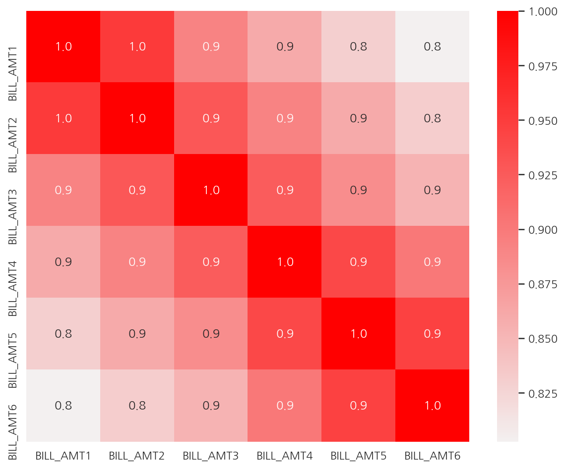
피처 간 상관관계를 확인하였을 때 BILL_AMT1 ~ BILL_AMT6 간의 상관계수가 0.8 ~ 1.0으로 매우 높다.
여기선 전체 상관관계를 확인하고 피처 간 상관계수가 높은 피처에 대해서만 시각화 하였다.
전체를 보고 싶다면 주석 코드를 실행하자.

# 피처 스케일링 
scaler = StandardScaler()
df_cols_scaled = scaler.fit_transform(X_features[cols_bill])

# PCA: n = 2
pca = PCA(n_components=2)
pca.fit(df_cols_scaled) 

print('PCA Component별 변동성:', pca.explained_variance_ratio_)

PCA Component별 변동성: [0.90555253 0.0509867 ]

앞서 상관계수가 높은 피처 BILL_AMT1 ~ BILL_AMT6을 스케일링 후 PCA 변환하였다.
2개의 PCA 컴포넌트만으로 6개 속성의 변동성을 약 95% 설명 가능하다.
특히 첫 번째 PCA 축으로 90%의 변동성을 설명할 정도로 기존 6개 속성의 상관도가 매우 높다.

PCA 변환 전 성능

from sklearn.ensemble import RandomForestClassifier
from sklearn.model_selection import cross_val_score

# 분류 모델: 랜덤 포레스트
rcf = RandomForestClassifier(n_estimators=300, random_state=1017)

# 교차 검증
scores = cross_val_score(rcf, X_features, y_target, scoring='accuracy', cv=3 )

print(f"원본 데이터 fold별 정확도: {scores}")
print(f"원본 데이터 평균 정확도: {np.mean(scores):.4f}")

원본 데이터 fold별 정확도: [0.8082 0.8217 0.8223]
원본 데이터 평균 정확도: 0.8174

from sklearn.decomposition import PCA
from sklearn.preprocessing import StandardScaler

# 피처 스케일링
scaler = StandardScaler()
df_scaled = scaler.fit_transform(X_features)

# PCA: n = 6
pca = PCA(n_components=6)
df_pca = pca.fit_transform(df_scaled)

# 분류 모델: 랜덤 포레스트
rcf = RandomForestClassifier(n_estimators=300, random_state=1017)

# 교차 검증
pca_scores = cross_val_score(rcf, df_pca, y_target, scoring='accuracy', cv=3)

print(f"PCA 데이터 fold별 정확도: {pca_scores}")
print(f"PCA 데이터 평균 정확도: {np.mean(pca_scores):.4f}")

PCA 데이터 fold별 정확도: [0.792  0.7976 0.8036]
PCA 데이터 평균 정확도: 0.7977

PCA 변환 전 23개의 속성에서 약 25% 수준인 6개의 PCA 컴포넌트로 예측하였음에도 정확도는 약 2%만 감소하였다.
2% 감소가 작은 것은 아니지만 전체 속성의 25%만으로도 이정도 예측 성능을 유지하는 것은 PCA의 압축 능력을 잘 보여준다.

Share on

Twitter Facebook LinkedIn

Romg2

[Python] 머신러닝 완벽가이드 - 06. 차원축소[PCA]

2. PCA(Principal Component Analysis)

2.1 IRIS 데이터

2.2 PCA 변환 전/후 분류

2.3 UCI 신용카드 고객 데이터

Share on

Leave a comment

You may also enjoy

[OPGG] 인턴 연계 과정 - 미니맵 챔피언 인식

[OPGG] 인턴 연계 과정 - 프로 리그 데이터 수집

[OPGG] 파이널 프로젝트 - 포지션 예측

[Python] 코딩 도장 - ASCII Art N

	sepal_length	sepal_width	petal_length	petal_width
0	5.1	3.5	1.4	0.2
1	4.9	3.0	1.4	0.2
2	4.7	3.2	1.3	0.2
3	4.6	3.1	1.5	0.2
4	5.0	3.6	1.4	0.2

	sepal_length	sepal_width	petal_length	petal_width
0	5.1	3.5	1.4	0.2
1	4.9	3.0	1.4	0.2
2	4.7	3.2	1.3	0.2
3	4.6	3.1	1.5	0.2
4	5.0	3.6	1.4	0.2

	sepal_length	sepal_width	petal_length	petal_width
0	5.1	3.5	1.4	0.2
1	4.9	3.0	1.4	0.2
2	4.7	3.2	1.3	0.2
3	4.6	3.1	1.5	0.2
4	5.0	3.6	1.4	0.2