
[Python] 머신러닝 완벽가이드 - 04. 분류[실습]
Updated:
파이썬 머신러닝 완벽가이드 교재를 토대로 공부한 내용입니다.
실습과정에서 필요에 따라 내용의 누락 및 추가, 수정사항이 있습니다.
기본 세팅
import numpy as np
import pandas as pd

import matplotlib as mpl
import matplotlib.pyplot as plt
import seaborn as sns

import warnings
%matplotlib inline
%config InlineBackend.figure_format = 'retina'

mpl.rc('font', family='NanumGothic') # 폰트 설정
mpl.rc('axes', unicode_minus=False) # 유니코드에서 음수 부호 설정

# 차트 스타일 설정
sns.set(font="NanumGothic", rc={"axes.unicode_minus":False}, style='darkgrid')
plt.rc("figure", figsize=(10,8))

warnings.filterwarnings("ignore")
1. 캐글 산탄데르 고객 만족 예측
산탄데르 은행이 캐글에 경연을 의뢰한 데이터로 피처 이름은 모두 익명 처리돼 이름만을 가지고 어떤 속성인지는 알 수 없다.
레이블 값은 1이면 불만을 가진 고객, 0이면 만족한 고객이다.
1.1 데이터 불러오기 및 전처리
cust_df = pd.read_csv("./santander_customer_satisfaction/train.csv", encoding="latin-1")
cust_df.head()
| ID | var3 | var15 | imp_ent_var16_ult1 | imp_op_var39_comer_ult1 | imp_op_var39_comer_ult3 | imp_op_var40_comer_ult1 | imp_op_var40_comer_ult3 | imp_op_var40_efect_ult1 | imp_op_var40_efect_ult3 | ... | saldo_medio_var33_hace2 | saldo_medio_var33_hace3 | saldo_medio_var33_ult1 | saldo_medio_var33_ult3 | saldo_medio_var44_hace2 | saldo_medio_var44_hace3 | saldo_medio_var44_ult1 | saldo_medio_var44_ult3 | var38 | TARGET | |
|---|---|---|---|---|---|---|---|---|---|---|---|---|---|---|---|---|---|---|---|---|---|
| 0 | 1 | 2 | 23 | 0.0 | 0.0 | 0.0 | 0.0 | 0.0 | 0.0 | 0.0 | ... | 0.0 | 0.0 | 0.0 | 0.0 | 0.0 | 0.0 | 0.0 | 0.0 | 39205.170000 | 0 |
| 1 | 3 | 2 | 34 | 0.0 | 0.0 | 0.0 | 0.0 | 0.0 | 0.0 | 0.0 | ... | 0.0 | 0.0 | 0.0 | 0.0 | 0.0 | 0.0 | 0.0 | 0.0 | 49278.030000 | 0 |
| 2 | 4 | 2 | 23 | 0.0 | 0.0 | 0.0 | 0.0 | 0.0 | 0.0 | 0.0 | ... | 0.0 | 0.0 | 0.0 | 0.0 | 0.0 | 0.0 | 0.0 | 0.0 | 67333.770000 | 0 |
| 3 | 8 | 2 | 37 | 0.0 | 195.0 | 195.0 | 0.0 | 0.0 | 0.0 | 0.0 | ... | 0.0 | 0.0 | 0.0 | 0.0 | 0.0 | 0.0 | 0.0 | 0.0 | 64007.970000 | 0 |
| 4 | 10 | 2 | 39 | 0.0 | 0.0 | 0.0 | 0.0 | 0.0 | 0.0 | 0.0 | ... | 0.0 | 0.0 | 0.0 | 0.0 | 0.0 | 0.0 | 0.0 | 0.0 | 117310.979016 | 0 |
5 rows × 371 columns
cust_df.info()
print("결측값의 수:", cust_df.isna().sum().sum())
print("타겟 type:", cust_df.TARGET.dtype)
<class 'pandas.core.frame.DataFrame'>
RangeIndex: 76020 entries, 0 to 76019
Columns: 371 entries, ID to TARGET
dtypes: float64(111), int64(260)
memory usage: 215.2 MB
결측값의 수: 0
타겟 type: int64
-
76,020개의 행, 371개의 열로 이루어져있으며 결측값은 없다.
-
370개의 피처 중 float형이 111개, int형이 259개이다.
cust_df.describe()
| ID | var3 | var15 | imp_ent_var16_ult1 | imp_op_var39_comer_ult1 | imp_op_var39_comer_ult3 | imp_op_var40_comer_ult1 | imp_op_var40_comer_ult3 | imp_op_var40_efect_ult1 | imp_op_var40_efect_ult3 | ... | saldo_medio_var33_hace2 | saldo_medio_var33_hace3 | saldo_medio_var33_ult1 | saldo_medio_var33_ult3 | saldo_medio_var44_hace2 | saldo_medio_var44_hace3 | saldo_medio_var44_ult1 | saldo_medio_var44_ult3 | var38 | TARGET | |
|---|---|---|---|---|---|---|---|---|---|---|---|---|---|---|---|---|---|---|---|---|---|
| count | 76020.000000 | 76020.000000 | 76020.000000 | 76020.000000 | 76020.000000 | 76020.000000 | 76020.000000 | 76020.000000 | 76020.000000 | 76020.000000 | ... | 76020.000000 | 76020.000000 | 76020.000000 | 76020.000000 | 76020.000000 | 76020.000000 | 76020.000000 | 76020.000000 | 7.602000e+04 | 76020.000000 |
| mean | 75964.050723 | -1523.199277 | 33.212865 | 86.208265 | 72.363067 | 119.529632 | 3.559130 | 6.472698 | 0.412946 | 0.567352 | ... | 7.935824 | 1.365146 | 12.215580 | 8.784074 | 31.505324 | 1.858575 | 76.026165 | 56.614351 | 1.172358e+05 | 0.039569 |
| std | 43781.947379 | 39033.462364 | 12.956486 | 1614.757313 | 339.315831 | 546.266294 | 93.155749 | 153.737066 | 30.604864 | 36.513513 | ... | 455.887218 | 113.959637 | 783.207399 | 538.439211 | 2013.125393 | 147.786584 | 4040.337842 | 2852.579397 | 1.826646e+05 | 0.194945 |
| min | 1.000000 | -999999.000000 | 5.000000 | 0.000000 | 0.000000 | 0.000000 | 0.000000 | 0.000000 | 0.000000 | 0.000000 | ... | 0.000000 | 0.000000 | 0.000000 | 0.000000 | 0.000000 | 0.000000 | 0.000000 | 0.000000 | 5.163750e+03 | 0.000000 |
| 25% | 38104.750000 | 2.000000 | 23.000000 | 0.000000 | 0.000000 | 0.000000 | 0.000000 | 0.000000 | 0.000000 | 0.000000 | ... | 0.000000 | 0.000000 | 0.000000 | 0.000000 | 0.000000 | 0.000000 | 0.000000 | 0.000000 | 6.787061e+04 | 0.000000 |
| 50% | 76043.000000 | 2.000000 | 28.000000 | 0.000000 | 0.000000 | 0.000000 | 0.000000 | 0.000000 | 0.000000 | 0.000000 | ... | 0.000000 | 0.000000 | 0.000000 | 0.000000 | 0.000000 | 0.000000 | 0.000000 | 0.000000 | 1.064092e+05 | 0.000000 |
| 75% | 113748.750000 | 2.000000 | 40.000000 | 0.000000 | 0.000000 | 0.000000 | 0.000000 | 0.000000 | 0.000000 | 0.000000 | ... | 0.000000 | 0.000000 | 0.000000 | 0.000000 | 0.000000 | 0.000000 | 0.000000 | 0.000000 | 1.187563e+05 | 0.000000 |
| max | 151838.000000 | 238.000000 | 105.000000 | 210000.000000 | 12888.030000 | 21024.810000 | 8237.820000 | 11073.570000 | 6600.000000 | 6600.000000 | ... | 50003.880000 | 20385.720000 | 138831.630000 | 91778.730000 | 438329.220000 | 24650.010000 | 681462.900000 | 397884.300000 | 2.203474e+07 | 1.000000 |
8 rows × 371 columns
-
var3의 경우 최소값이 -999999이다. 이는 NaN값이나 특정 예외 값을 변환한 것으로 판단된다.
-
ID의 경우 단순 식별자이므로 필요 없다.
print(cust_df.var3.value_counts().sort_index()[:1])
-999999    116
Name: var3, dtype: int64
- -999999가 116개가 존재하며 다른 값에 비해 std가 심하므로 최빈값으로 변환한다.
from scipy.stats import mode

# var3 최빈값
var3_mode = mode(cust_df.var3.values)[0][0]

# var3 대체, ID 제거
cust_df["var3"].replace(-999999, var3_mode, inplace=True)
cust_df.drop("ID", axis=1, inplace=True)
plt.figure(figsize=(10,5))

frequency = cust_df['TARGET'].value_counts()
label = [f"0: {frequency[0]}개", f"1: {frequency[1]}개"]

plt.pie(frequency,
    startangle = 180,
    counterclock = False,
    explode = [0.03] * 2,
    autopct = '%1.1f%%',
    labels = label,
    colors = sns.color_palette('pastel', 2),
    wedgeprops = dict(width=0.7)
  )


plt.axis('equal')
plt.show()
-
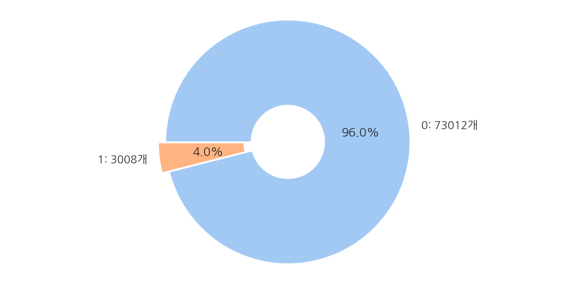
전체 76,020개 데이터 중 만족이 73,012개(96.0%), 불만족이 3,008개(4.0%)로 이루어져 있다.
-
대부분이 0(만족)이므로 정확도보다는 ROC-AUC로 성능을 평가한다.
1.2 성능 평가
from sklearn.model_selection import train_test_split

# 피처, 레이블 분리
X_features = cust_df.iloc[:,:-1]
y_label = cust_df.iloc[:,-1]

# train, test
X_train, X_test, y_train, y_test = train_test_split(X_features, y_label, test_size=0.2, random_state=0)

print("train 레이블 분포")
print(y_train.value_counts() / y_train.count() * 100)
print("-"*30)
print("test 레이블 분포")
print(y_test.value_counts() / y_test.count() * 100)
train 레이블 분포
0    96.096422
1     3.903578
Name: TARGET, dtype: float64
------------------------------
test 레이블 분포
0    95.830045
1     4.169955
Name: TARGET, dtype: float64
- train과 test 모두 레이블의 분포는 원 데이터와 유사하게 만들어졌다.
1.2.1 XGBoost
XGB 학습
from xgboost import XGBClassifier
from sklearn.metrics import roc_auc_score

# XGB 객체 생성
xgb_clf = XGBClassifier(n_estimators = 500, random_state = 156)

# 학습 - 조기 중단 설정, 성능 평가 AUC
evals = [ (X_train, y_train), (X_test, y_test)] # test set 사용은 과적합 주의
xgb_clf.fit(X_train, y_train,
            early_stopping_rounds=100, eval_metric="auc", eval_set=evals)
[0]	validation_0-auc:0.82005	validation_1-auc:0.81157
[1]	validation_0-auc:0.83400	validation_1-auc:0.82452
[2]	validation_0-auc:0.83870	validation_1-auc:0.82746
[3]	validation_0-auc:0.84419	validation_1-auc:0.82922
[4]	validation_0-auc:0.84783	validation_1-auc:0.83298
[5]	validation_0-auc:0.85125	validation_1-auc:0.83500
[6]	validation_0-auc:0.85501	validation_1-auc:0.83653
[7]	validation_0-auc:0.85830	validation_1-auc:0.83782
[8]	validation_0-auc:0.86143	validation_1-auc:0.83802
[9]	validation_0-auc:0.86452	validation_1-auc:0.83914
[10]	validation_0-auc:0.86717	validation_1-auc:0.83954
...
[111]	validation_0-auc:0.93663	validation_1-auc:0.82620
[112]	validation_0-auc:0.93710	validation_1-auc:0.82591
[113]	validation_0-auc:0.93781	validation_1-auc:0.82498
[114]	validation_0-auc:0.93793	validation_1-auc:0.82525


XGBClassifier(base_score=0.5, booster='gbtree', colsample_bylevel=1,
              colsample_bynode=1, colsample_bytree=1, gamma=0, gpu_id=-1,
              importance_type='gain', interaction_constraints='',
              learning_rate=0.300000012, max_delta_step=0, max_depth=6,
              min_child_weight=1, missing=nan, monotone_constraints='()',
              n_estimators=500, n_jobs=8, num_parallel_tree=1, random_state=156,
              reg_alpha=0, reg_lambda=1, scale_pos_weight=1, subsample=1,
              tree_method='exact', validate_parameters=1, verbosity=None)
-
n_estimators를 500으로 설정하였고 평가 set으로 train과 test를 사용하였을 때 114번 반복 후 조기 중단 되었다.
-
결과창이 너무 길어 직접 삭제하였다.
XGB 예측/평가
# 예측 확률
xgb_pred_proba = xgb_clf.predict_proba(X_test)[:,1].reshape(-1,1)

# 평가
xgb_roc_auc = roc_auc_score(y_test, xgb_pred_proba, average="macro")
print(f"AUC: {xgb_roc_auc:.4f}")
AUC: 0.8413
- test set으로 예측시 AUC는 약 0.8413으로 나타났다.
XGB GridSearchCV
from sklearn.model_selection import GridSearchCV

# XGB 객체 생성 - n_estimators 감소
xgb_clf2 = XGBClassifier(n_estimators = 100, random_state = 156)

# 하이퍼 파라미터
params = {
    "max_depth": [5, 7], # 깊이
    "min_child_weight": [1, 3], # 가지 분할 가중치
    "colsample_bytree": [0.5, 0.75] # 피처 선택 비율
}

# GridSearchCV
evals = [ (X_train, y_train), (X_test, y_test)] # test set 사용은 과적합 주의

grid_cv = GridSearchCV(xgb_clf2, param_grid=params, cv=3)
grid_cv.fit(X_train, y_train,
            early_stopping_rounds=100, eval_metric="auc", eval_set=evals)
GridSearchCV(cv=3,
             estimator=XGBClassifier(base_score=None, booster=None,
                                     colsample_bylevel=None,
                                     colsample_bynode=None,
                                     colsample_bytree=None, gamma=None,
                                     gpu_id=None, importance_type='gain',
                                     interaction_constraints=None,
                                     learning_rate=None, max_delta_step=None,
                                     max_depth=None, min_child_weight=None,
                                     missing=nan, monotone_constraints=None,
                                     n_estimators=100, n_jobs=None,
                                     num_parallel_tree=None, random_state=156,
                                     reg_alpha=None, reg_lambda=None,
                                     scale_pos_weight=None, subsample=None,
                                     tree_method=None, validate_parameters=None,
                                     verbosity=None),
             param_grid={'colsample_bytree': [0.5, 0.75], 'max_depth': [5, 7],
                         'min_child_weight': [1, 3]})
- 결과창이 너무 길어 직접 삭제하였다.
# 최적 하이퍼 파라미터
print("GridSearchCV 최적 하이퍼 파라미터:", grid_cv.best_params_)

# 최적 하이퍼 파라미터로 예측 평가
best_xgb_clf = grid_cv.best_estimator_
best_pred_proba = best_xgb_clf.predict_proba(X_test)[:,1].reshape(-1,1)
best_roc_auc = roc_auc_score(y_test, best_pred_proba, average="macro")
print(f"GridSearchCV AUC: {best_roc_auc:.4f}")
GridSearchCV 최적 하이퍼 파라미터: {'colsample_bytree': 0.5, 'max_depth': 7, 'min_child_weight': 1}
GridSearchCV AUC: 0.8429
-
최적 하이퍼 파라미터는 colsample_bytree: 0.5, max_depth: 7, min_child_weight: 1 이고, 이때 AUC는 0.8429이다.
-
앞서 AUC가 0.8413에서 미미하지만 조금 증가하였다.
-
수행시간이 확실히 오래 걸린다.
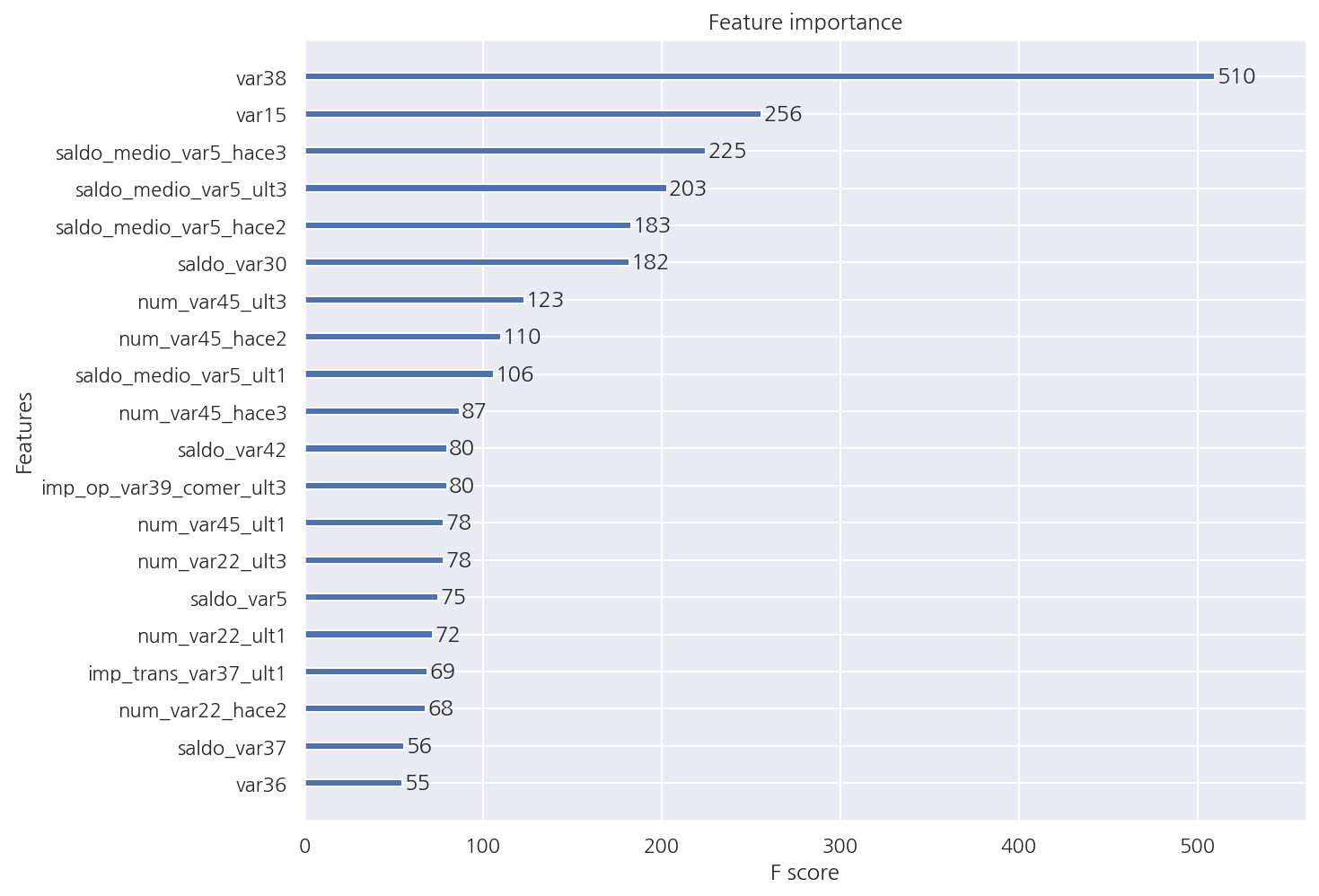
XGB 피처별 중요도
from xgboost import plot_importance

plot_importance(best_xgb_clf, max_num_features=20)
plt.show()
1.2.2 LightGBM
LGBM 학습
from lightgbm import LGBMClassifier

# LGBM 객체 생성
lgbm_clf = LGBMClassifier(n_estimators = 500, random_state = 156)

# 학습 - 조기 중단 설정, 성능 평가 AUC
evals = [ (X_test, y_test) ] # test set 사용은 과적합 주의
lgbm_clf.fit(X_train, y_train,
             early_stopping_rounds=100, eval_metric="auc", eval_set=evals,
             verbose=True)
[1]	valid_0's auc: 0.817384	valid_0's binary_logloss: 0.165046
Training until validation scores don't improve for 100 rounds
[2]	valid_0's auc: 0.818903	valid_0's binary_logloss: 0.160006
...
[15]	valid_0's auc: 0.840928	valid_0's binary_logloss: 0.14161
...
[111]	valid_0's auc: 0.836957	valid_0's binary_logloss: 0.140426
[112]	valid_0's auc: 0.836779	valid_0's binary_logloss: 0.14051
[113]	valid_0's auc: 0.836831	valid_0's binary_logloss: 0.140526
[114]	valid_0's auc: 0.836783	valid_0's binary_logloss: 0.14055
[115]	valid_0's auc: 0.836672	valid_0's binary_logloss: 0.140585
Early stopping, best iteration is:
[15]	valid_0's auc: 0.840928	valid_0's binary_logloss: 0.14161


LGBMClassifier(n_estimators=500, random_state=156)
-
115번 반복 후 조기 중단되었다.
-
결과창이 너무 길어 직접 삭제하였다.
LGBM 예측/평가
# 예측 확률
lgbm_pred_proba = lgbm_clf.predict_proba(X_test)[:,1].reshape(-1,1)

# 평가
lgbm_roc_auc = roc_auc_score(y_test, lgbm_pred_proba, average="macro")
print(f"AUC: {lgbm_roc_auc:.4f}")
AUC: 0.8409
- AUC는 0.8409로 XGB로 수행하였을 때보다는 작은 수치로 나타났다.
LGBM GridSearchCV
from sklearn.model_selection import GridSearchCV

# LGBM 객체 생성 - n_estimators 감소
lgbm_clf2 = LGBMClassifier(n_estimators = 200, random_state = 156)

# 하이퍼 파라미터
params = {
    "num_leaves": [32, 64], # 최대 리프 수
    "max_depth": [128, 160], # 깊이
    "min_child_samples": [60, 100], # 리프 최소 샘플 수
    "subsample": [0.8, 1] # 샘플 비율
}

# GridSearchCV
evals = [ (X_train, y_train), (X_test, y_test) ] # test set 사용은 과적합 주의

grid_cv2 = GridSearchCV(lgbm_clf2, param_grid=params, cv=3)
grid_cv2.fit(X_train, y_train,
             early_stopping_rounds=100, eval_metric="auc", eval_set=evals)
GridSearchCV(cv=3, estimator=LGBMClassifier(n_estimators=200, random_state=156),
             param_grid={'max_depth': [128, 160],
                         'min_child_samples': [60, 100], 'num_leaves': [32, 64],
                         'subsample': [0.8, 1]})
- 결과창이 너무 길어 직접 삭제하였다.
# 최적 하이퍼 파라미터
print("GridSearchCV 최적 하이퍼 파라미터:", grid_cv2.best_params_)

# 최적 하이퍼 파라미터로 예측 평가
best_lgbm_clf = grid_cv2.best_estimator_
best_pred_proba2 = best_lgbm_clf.predict_proba(X_test)[:,1].reshape(-1,1)
best_roc_auc2 = roc_auc_score(y_test, best_pred_proba2, average="macro")
print(f"GridSearchCV AUC: {best_roc_auc2:.4f}")
GridSearchCV 최적 하이퍼 파라미터: {'max_depth': 128, 'min_child_samples': 100, 'num_leaves': 32, 'subsample': 0.8}
GridSearchCV AUC: 0.8417
-
앞서 AUC가 0.8409에서 0.8417로 조금 증가하였고 GridSearchCV로 XGB를 수행하였을 때 0.8429 보단 작게 나타났다.
-
수행시간은 확실 XGB보다도 훨씬 빠른 것이 체감된다.
2. 캐글 신용카드 사기 검출
데이터의 레이블인 Class는 1이면 신용카드 사기 트랜잭션, 0이면 정상적인 신용카드 트랜잭션 데이터다.
전체 데이터의 약 0.172%만이 1, 사기 트랜잭션으로 레이블은 매우 불균형한 분포다.
일반적으로 사기 검출, 이상 검출과 같은 데이터는 이처럼 매우 불균형한 분포일 가능성이 높을 수 밖에 없다.
2.1 언더 샘플링, 오버 샘플링
현 예제처럼 극도로 불균형한 레이블 값 분포로 인한 문제점을 해결하기 위해서는 적절한 학습 데이터를 확보하는 방안이 필요하다.
대표적으로 언더 샘플링과 오버 샘플링이 있으며 오버 샘플링 방식이 예측 성능상 더 유리한 경우가 많아 주로 사용된다.
언더 샘플링
-
많은 데이터 셋을 적은 데이터 셋 수준으로 감소시키는 방식
-
정상 레이블이 10,000건, 이상 레이블이 100건이라면 정상 레이블 데이터를 100건으로 줄여버린다.
-
기존보다 과도하게 정상 레이블로 학습/예측하는 부작용은 개선되지만 과도한 데이터 감소로 정상 레이블의 경우 오히려 제대로 된 학습 수행을 할 수 없다.
오버 샘플링
-
적은 데이터 셋을 많은 데이터 셋 수준으로 증가시키는 방식
-
단순히 동일한 데이터를 증식하면 과적합이 되기에 원본 데이터의 피처 값을 약간만 변경하여 증식한다.
-
대표적으로 SMOTE(Synthetic Minority Over-sampling Technique) 방법이 있다.
-
SMOTE는 적은 데이터 셋에 있는 개별 데이터들의 K 최근접 이웃(KNN)을 찾아 데이터와 K개의 이웃들의 차이를 일정 값으로 만들어 기존 데이터와 약간 차이가 나는 새로운 데이터들을 생성하는 방식이다.
2.2 데이터 1차 가공 및 학습/예측/평가
2.2.1 데이터 1차 가공
card_df = pd.read_csv("./creditcard.csv")
card_df.head()
| Time | V1 | V2 | V3 | V4 | V5 | V6 | V7 | V8 | V9 | ... | V21 | V22 | V23 | V24 | V25 | V26 | V27 | V28 | Amount | Class | |
|---|---|---|---|---|---|---|---|---|---|---|---|---|---|---|---|---|---|---|---|---|---|
| 0 | 0.0 | -1.359807 | -0.072781 | 2.536347 | 1.378155 | -0.338321 | 0.462388 | 0.239599 | 0.098698 | 0.363787 | ... | -0.018307 | 0.277838 | -0.110474 | 0.066928 | 0.128539 | -0.189115 | 0.133558 | -0.021053 | 149.62 | 0 |
| 1 | 0.0 | 1.191857 | 0.266151 | 0.166480 | 0.448154 | 0.060018 | -0.082361 | -0.078803 | 0.085102 | -0.255425 | ... | -0.225775 | -0.638672 | 0.101288 | -0.339846 | 0.167170 | 0.125895 | -0.008983 | 0.014724 | 2.69 | 0 |
| 2 | 1.0 | -1.358354 | -1.340163 | 1.773209 | 0.379780 | -0.503198 | 1.800499 | 0.791461 | 0.247676 | -1.514654 | ... | 0.247998 | 0.771679 | 0.909412 | -0.689281 | -0.327642 | -0.139097 | -0.055353 | -0.059752 | 378.66 | 0 |
| 3 | 1.0 | -0.966272 | -0.185226 | 1.792993 | -0.863291 | -0.010309 | 1.247203 | 0.237609 | 0.377436 | -1.387024 | ... | -0.108300 | 0.005274 | -0.190321 | -1.175575 | 0.647376 | -0.221929 | 0.062723 | 0.061458 | 123.50 | 0 |
| 4 | 2.0 | -1.158233 | 0.877737 | 1.548718 | 0.403034 | -0.407193 | 0.095921 | 0.592941 | -0.270533 | 0.817739 | ... | -0.009431 | 0.798278 | -0.137458 | 0.141267 | -0.206010 | 0.502292 | 0.219422 | 0.215153 | 69.99 | 0 |
5 rows × 31 columns
-
Time 피처는 데이터 생성 관련 작업용 속성으로 큰 의미가 없어 제거한다.
-
V1 ~ V28은 피처의 의미를 알 수 없으며 Amount 피처는 신용카드 트랜잭션 금액을 의미한다.
card_df.info()
<class 'pandas.core.frame.DataFrame'>
RangeIndex: 284807 entries, 0 to 284806
Data columns (total 31 columns):
 #   Column  Non-Null Count   Dtype
---  ------  --------------   -----
 0   Time    284807 non-null  float64
 1   V1      284807 non-null  float64
 2   V2      284807 non-null  float64
 3   V3      284807 non-null  float64
 4   V4      284807 non-null  float64
 5   V5      284807 non-null  float64
 6   V6      284807 non-null  float64
 7   V7      284807 non-null  float64
 8   V8      284807 non-null  float64
 9   V9      284807 non-null  float64
 10  V10     284807 non-null  float64
 11  V11     284807 non-null  float64
 12  V12     284807 non-null  float64
 13  V13     284807 non-null  float64
 14  V14     284807 non-null  float64
 15  V15     284807 non-null  float64
 16  V16     284807 non-null  float64
 17  V17     284807 non-null  float64
 18  V18     284807 non-null  float64
 19  V19     284807 non-null  float64
 20  V20     284807 non-null  float64
 21  V21     284807 non-null  float64
 22  V22     284807 non-null  float64
 23  V23     284807 non-null  float64
 24  V24     284807 non-null  float64
 25  V25     284807 non-null  float64
 26  V26     284807 non-null  float64
 27  V27     284807 non-null  float64
 28  V28     284807 non-null  float64
 29  Amount  284807 non-null  float64
 30  Class   284807 non-null  int64
dtypes: float64(30), int64(1)
memory usage: 67.4 MB
-
284,807개의 행, 31개의 열로 이루어져있으며 결측값은 없다.
-
레이블을 제외한 피처는 모두 float형이다.
데이터 가공 함수
from sklearn.model_selection import train_test_split

# DF 복사 후 Time 컬럼 삭제하고 복사된 DF 반환
def get_preprocessed_df(df=None):
    df_copy = df.copy()
    df_copy.drop("Time", axis=1, inplace=True)
    return df_copy

# 데이터 가공 후 train, test 반환
def get_train_test_dataset(df=None):
    temp_df = get_preprocessed_df(df)

    # 피처, 레이블 분리
    X_features = temp_df.iloc[:,:-1]
    y_target = temp_df.iloc[:,-1]

    # train, test 생성, 원 데이터 분포 반영
    X_train, X_test, y_train, y_test = train_test_split(X_features, y_target,
                                                        test_size=0.3, random_state=0, stratify=y_target)

    return X_train, X_test, y_train, y_test
X_train, X_test, y_train, y_test = get_train_test_dataset(card_df)
print("train 레이블 분포")
print(y_train.value_counts() / y_train.count() * 100)
print("-"*30)
print("test 레이블 분포")
print(y_test.value_counts() / y_test.count() * 100)
train 레이블 분포
0    99.827451
1     0.172549
Name: Class, dtype: float64
------------------------------
test 레이블 분포
0    99.826785
1     0.173215
Name: Class, dtype: float64
- train과 test 모두 레이블의 분포는 원 데이터와 유사하게 만들어졌다.
2.2.2 성능 평가
# 3장에서 사용한 성능 평가 함수
from sklearn.metrics import accuracy_score, precision_score, recall_score, confusion_matrix
from sklearn.metrics import f1_score, roc_auc_score

def get_clf_eval(y_test, pred=None, pred_proba_po=None):
    confusion = confusion_matrix(y_test, pred)
    accuracy = accuracy_score(y_test, pred)
    precision = precision_score(y_test, pred)
    recall = recall_score(y_test, pred)
    f1 = f1_score(y_test, pred)
    auc = roc_auc_score(y_test, pred_proba_po)

    print("오차 행렬")
    print(confusion)
    print(f"정확도: {accuracy:.4f}, 정밀도: {precision:.4f}, 재현율: {recall:.4f}, F1: {f1:.4f}, AUC: {auc:.4f}")
# 학습/예측/평가 함수
def get_model_train_eval(model, train_x=None, test_x=None, train_y=None, test_y=None):
    model.fit(train_x, train_y)
    pred = model.predict(test_x)
    pred_proba = model.predict_proba(test_x)[:,1].reshape(-1,1)
    get_clf_eval(test_y, pred, pred_proba)
2.2.2.1 Logistic Regression
from sklearn.linear_model import LogisticRegression

lr_clf = LogisticRegression()
get_model_train_eval(lr_clf, train_x=X_train, test_x=X_test, train_y=y_train, test_y=y_test)
오차 행렬
[[85282    13]
 [   56    92]]
정확도: 0.9992, 정밀도: 0.8762, 재현율: 0.6216, F1: 0.7273, AUC: 0.9586
2.2.2.2 LightGBM
import lightgbm
lightgbm.__version__
'3.2.1'
-
LightGBM 2.1.0 이상 버전에서 boost_from_average 파라미터 디폴트 값은 True이다.
-
레이블 값이 극도로 불균형한 분포인 경우 boost_from_average를 True로 설정하면 재현율, AUC 성능을 저하 한다고 한다.
from lightgbm import LGBMClassifier

lgbm_clf3 = LGBMClassifier(n_estimators=1000, num_leaves=64, n_jobs=-1)
get_model_train_eval(lgbm_clf3, train_x=X_train, test_x=X_test, train_y=y_train, test_y=y_test)
오차 행렬
[[85224    71]
 [   83    65]]
정확도: 0.9982, 정밀도: 0.4779, 재현율: 0.4392, F1: 0.4577, AUC: 0.7225
-
boost_from_average = True인 경우 확실히 정밀도, 재현율, F1, AUC 모두 크게 저하되어있다.
-
이에 대해선 따로 공부해야겠다.
from lightgbm import LGBMClassifier

lgbm_clf3 = LGBMClassifier(n_estimators=1000, num_leaves=64, n_jobs=-1, boost_from_average=False)
get_model_train_eval(lgbm_clf3, train_x=X_train, test_x=X_test, train_y=y_train, test_y=y_test)
오차 행렬
[[85290     5]
 [   36   112]]
정확도: 0.9995, 정밀도: 0.9573, 재현율: 0.7568, F1: 0.8453, AUC: 0.9790
-
boost_from_average = False로 설정하니 True에 비해 성능이 확실히 좋게 나왔다.
-
로지스틱에 비해서 성능이 향상된 것이 확인된다.
2.3 데이터 분포 변환 및 학습/예측/평가
2.3.1 데이터 분포 변환
card_df.describe()[["Amount"]].T
| count | mean | std | min | 25% | 50% | 75% | max | |
|---|---|---|---|---|---|---|---|---|
| Amount | 284807.0 | 88.349619 | 250.120109 | 0.0 | 5.6 | 22.0 | 77.165 | 25691.16 |
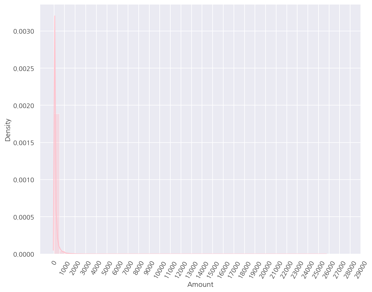
- Amount는 평균값이 약 88이고 3분위수도 77인데 최대값은 25,691로 매우 크다.
sns.distplot(card_df.Amount, kde = True, color = "pink")
plt.xticks( range(0, 30000, 1000), rotation=60)
plt.show()
-
분포를 확인하였을 때 사용금액이 1,000불 이하가 대부분이며 일부만 매우 큰 금액임을 알 수 있다.
-
로지스틱 회귀 등 대부분 선형 모델은 피처가 정규 분포 형태를 띄는 것을 선호하므로 추가적으로 가공을 진행한다.
데이터 가공 함수
from sklearn.model_selection import train_test_split
from sklearn.preprocessing import StandardScaler

# DF 복사 후 Time 컬럼 삭제하고 복사된 DF 반환 + Amount 스케일링
def get_preprocessed_df(df=None):
    df_copy = df.copy()

    # Amount 스케일링
    scaler = StandardScaler()
    amount_scaled = scaler.fit_transform(df_copy.Amount.values.reshape(-1,1))
    df_copy.Amount = amount_scaled

    df_copy.drop("Time", axis=1, inplace=True)
    return df_copy

# 데이터 가공 후 train, test 반환
def get_train_test_dataset(df=None):
    temp_df = get_preprocessed_df(df)

    # 피처, 레이블 분리
    X_features = temp_df.iloc[:,:-1]
    y_target = temp_df.iloc[:,-1]

    # train, test 생성, 원 데이터 분포 반영
    X_train, X_test, y_train, y_test = train_test_split(X_features, y_target,
                                                        test_size=0.3, random_state=0, stratify=y_target)

    return X_train, X_test, y_train, y_test
2.3.2 성능 평가
# Amount 스케일링 후 데이터 셋 생성
X_train, X_test, y_train, y_test = get_train_test_dataset(card_df)

# Logistic Regression 성능 평가
print("### Logistic Regression 성능 평가")
lr_clf2 = LogisticRegression()
get_model_train_eval(lr_clf2, train_x=X_train, test_x=X_test, train_y=y_train, test_y=y_test)

# LightGBM 성능 평가
print("### LightGBM 성능 평가")
lgbm_clf4 = LGBMClassifier(n_estimators=1000, num_leaves=64, n_jobs=-1, boost_from_average=False)
get_model_train_eval(lgbm_clf4, train_x=X_train, test_x=X_test, train_y=y_train, test_y=y_test)
### Logistic Regression 성능 평가
오차 행렬
[[85281    14]
 [   58    90]]
정확도: 0.9992, 정밀도: 0.8654, 재현율: 0.6081, F1: 0.7143, AUC: 0.9702
### LightGBM 성능 평가
오차 행렬
[[85291     4]
 [   36   112]]
정확도: 0.9995, 정밀도: 0.9655, 재현율: 0.7568, F1: 0.8485, AUC: 0.9782
- Amount 스케일링 전후 성능 평가 지표의 차이는 크게 없다.
2.3.3 데이터 로그 변환
이번에는 StandardScaler가 아닌 로그 변환을 적용해본다.
로그 변환은 데이터 분포가 심하게 왜곡되어 있을 때 적용하는 중요 기법 중 하나로 변환 시 상대적으로 값이 작아지기에 데이터 분포 왜곡을 개선해준다.
데이터 가공 함수
from sklearn.model_selection import train_test_split
from sklearn.preprocessing import StandardScaler

# DF 복사 후 Time 컬럼 삭제하고 복사된 DF 반환 + Amount 로그 변환
def get_preprocessed_df(df=None):
    df_copy = df.copy()

    # Amount 로그 변환
    amount_log_scaled = np.log1p(df_copy.Amount)
    df_copy.Amount = amount_log_scaled

    df_copy.drop("Time", axis=1, inplace=True)
    return df_copy

# 데이터 가공 후 train, test 반환
def get_train_test_dataset(df=None):
    temp_df = get_preprocessed_df(df)

    # 피처, 레이블 분리
    X_features = temp_df.iloc[:,:-1]
    y_target = temp_df.iloc[:,-1]

    # train, test 생성, 원 데이터 분포 반영
    X_train, X_test, y_train, y_test = train_test_split(X_features, y_target,
                                                        test_size=0.3, random_state=0, stratify=y_target)

    return X_train, X_test, y_train, y_test
2.3.4 성능 평가
# Amount 로그 변환 후 데이터 셋 생성
X_train, X_test, y_train, y_test = get_train_test_dataset(card_df)

# Logistic Regression 성능 평가
print("### Logistic Regression 성능 평가")
lr_clf3 = LogisticRegression()
get_model_train_eval(lr_clf3, train_x=X_train, test_x=X_test, train_y=y_train, test_y=y_test)

# LightGBM 성능 평가
print("### LightGBM 성능 평가")
lgbm_clf5 = LGBMClassifier(n_estimators=1000, num_leaves=64, n_jobs=-1, boost_from_average=False)
get_model_train_eval(lgbm_clf5, train_x=X_train, test_x=X_test, train_y=y_train, test_y=y_test)
### Logistic Regression 성능 평가
오차 행렬
[[85283    12]
 [   59    89]]
정확도: 0.9992, 정밀도: 0.8812, 재현율: 0.6014, F1: 0.7149, AUC: 0.9727
### LightGBM 성능 평가
오차 행렬
[[85290     5]
 [   36   112]]
정확도: 0.9995, 정밀도: 0.9573, 재현율: 0.7568, F1: 0.8453, AUC: 0.9790
- Logistic Regression의 경우 대체로 성능이 향상되었고 LightGBM의 경우 큰 차이가 없다.
2.4 이상치 제거 및 학습/예측/평가
이번에는 이상치 데이터를 제거하고 학습/예측/평가를 진행해본다.
이상치 기준은 IQR 방식을 적용한다.
corr_M = card_df.corr()
sns.heatmap(corr_M, cmap="RdBu")
plt.show()
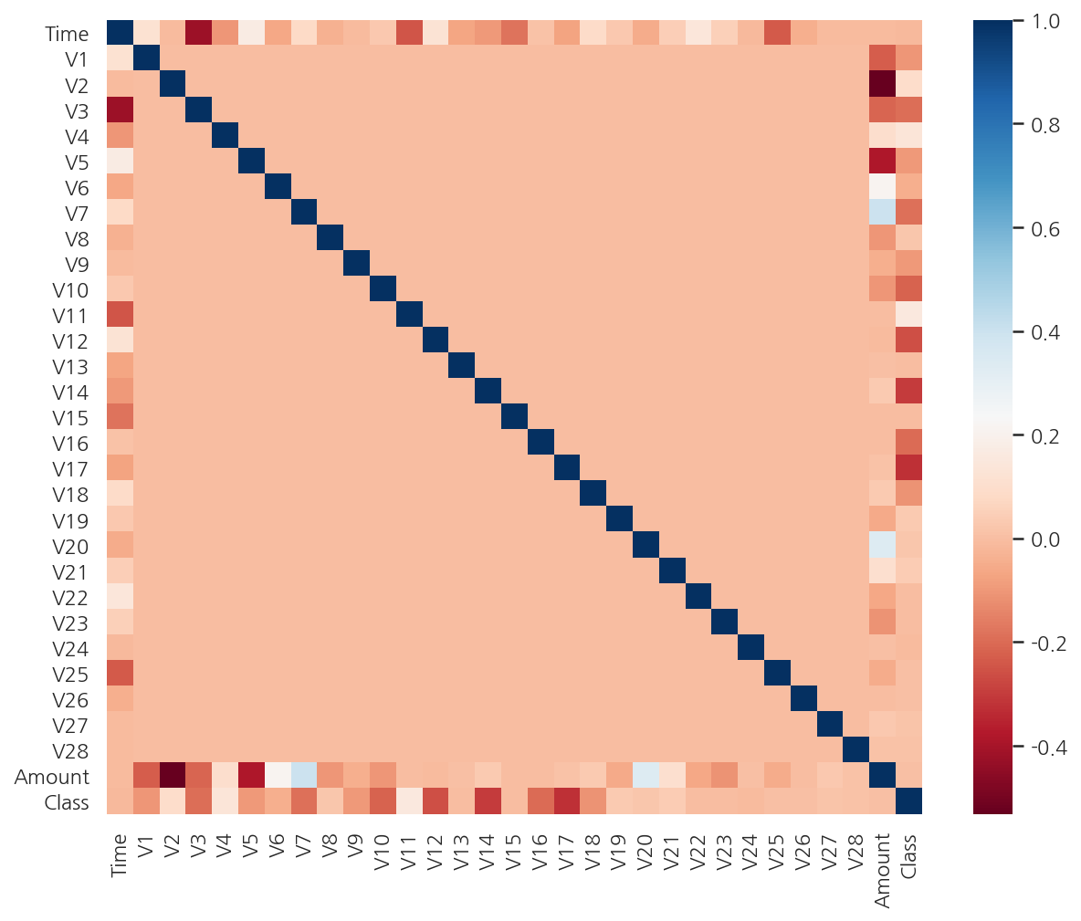
- 상관관계 히트맵에서 Class와 음의 상관관계가 높은 V14와 V17 중 V14에 대해서 이상치 제거를 작업해보기로 한다.
2.4.1 데이터 이상치 제거
# IQR 이상치 제거
def get_outlier(df=None, column=None):
    # Class가 1인 경우만 진행
    fraud = df[df.Class == 1][column]

    # IQR 및 Boundary 설정
    Q1 = np.percentile(fraud.values, 25)
    Q3 = np.percentile(fraud.values, 75)
    IQR = Q3 - Q1
    upper_bound = Q3 + 1.5 * IQR
    lower_bound = Q1 - 1.5 * IQR

    # 이상치 인덱스 반환
    outlier_index = fraud[ (fraud < lower_bound) | (fraud > upper_bound)].index
    return outlier_index

get_outlier(card_df, "V14")
Int64Index([8296, 8615, 9035, 9252], dtype='int64')
-
IQR 방식으로 이상치 인덱스를 반환하는 함수를 생성하였다.
-
이상치 인덱스는 Class가 1인 경우만 찾았다.
데이터 가공 함수
from sklearn.model_selection import train_test_split
from sklearn.preprocessing import StandardScaler

# Time 삭제후 DF 반환 + Amount 로그 변환 + 이상치 제거
def get_preprocessed_df(df=None):
    df_copy = df.copy()

    # Amount 로그 변환
    amount_log_scaled = np.log1p(df_copy.Amount)
    df_copy.Amount = amount_log_scaled

    # IQR 이상치 제거
    outlier_index = get_outlier(df_copy, "V14")
    df_copy.drop(outlier_index, axis=0, inplace=True)

    # Time 삭제
    df_copy.drop("Time", axis=1, inplace=True)
    return df_copy

# 데이터 가공 후 train, test 반환
def get_train_test_dataset(df=None):
    temp_df = get_preprocessed_df(df)

    # 피처, 레이블 분리
    X_features = temp_df.iloc[:,:-1]
    y_target = temp_df.iloc[:,-1]

    # train, test 생성, 원 데이터 분포 반영
    X_train, X_test, y_train, y_test = train_test_split(X_features, y_target,
                                                        test_size=0.3, random_state=0, stratify=y_target)

    return X_train, X_test, y_train, y_test
2.4.2 성능 평가
# 이상치 제거 추가 후 데이터 셋 생성
X_train, X_test, y_train, y_test = get_train_test_dataset(card_df)

# Logistic Regression 성능 평가
print("### Logistic Regression 성능 평가")
lr_clf4 = LogisticRegression()
get_model_train_eval(lr_clf4, train_x=X_train, test_x=X_test, train_y=y_train, test_y=y_test)

# LightGBM 성능 평가
print("### LightGBM 성능 평가")
lgbm_clf6 = LGBMClassifier(n_estimators=1000, num_leaves=64, n_jobs=-1, boost_from_average=False)
get_model_train_eval(lgbm_clf6, train_x=X_train, test_x=X_test, train_y=y_train, test_y=y_test)
### Logistic Regression 성능 평가
오차 행렬
[[85281    14]
 [   48    98]]
정확도: 0.9993, 정밀도: 0.8750, 재현율: 0.6712, F1: 0.7597, AUC: 0.9743
### LightGBM 성능 평가
오차 행렬
[[85291     4]
 [   25   121]]
정확도: 0.9997, 정밀도: 0.9680, 재현율: 0.8288, F1: 0.8930, AUC: 0.9791
- 이상치 제거 후 두 모델 모두 모든 예측 성능이 크게 향상 되었다.
2.5 SMOTE 오버 샘플링 및 학습/예측/평가
2.5.1 SMOTE 오버 샘플링
이번에는 SMOTE 오버 샘플링 후 학습/예측/평가를 진행해본다.
주의할 점은 SMOTE 오버 샘플링은 반드시 train set에만 적용하여야 한다.
from imblearn.over_sampling import SMOTE

smote = SMOTE(random_state=0)
X_train_over, y_train_over = smote.fit_sample(X_train, y_train)

print("SMOTE 적용 전 train 피처/레이블 shape", X_train.shape, y_train.shape)
print("SMOTE 적용 후 train 피처/레이블 shape", X_train_over.shape, y_train_over.shape)
print("-"*60)
print("SMOTE 적용 후 레이블 분포")
print(y_train_over.value_counts())
SMOTE 적용 전 train 피처/레이블 shape (199362, 29) (199362,)
SMOTE 적용 후 train 피처/레이블 shape (398040, 29) (398040,)
------------------------------------------------------------
SMOTE 적용 후 레이블 분포
1    199020
0    199020
Name: Class, dtype: int64
-
SMOTE 오버 샘플링 이후 데이터가 대략 2배 정도 증가하였다.
-
또한 레이블 값이 0과 1의 분포가 동일하게 생성되었다.
2.5.2 성능 평가
# 이상치 제거 추가 후 데이터 셋 생성
X_train, X_test, y_train, y_test = get_train_test_dataset(card_df)

# SMOTE 오버 샘플링
smote = SMOTE(random_state=0)
X_train_over, y_train_over = smote.fit_sample(X_train, y_train)

# Logistic Regression 성능 평가
print("### Logistic Regression 성능 평가")
lr_clf5 = LogisticRegression()
get_model_train_eval(lr_clf5, train_x=X_train_over, test_x=X_test, train_y=y_train_over, test_y=y_test)

# LightGBM 성능 평가
print("### LightGBM 성능 평가")
lgbm_clf7 = LGBMClassifier(n_estimators=1000, num_leaves=64, n_jobs=-1, boost_from_average=False)
get_model_train_eval(lgbm_clf7, train_x=X_train_over, test_x=X_test, train_y=y_train_over, test_y=y_test)
### Logistic Regression 성능 평가
오차 행렬
[[82937  2358]
 [   11   135]]
정확도: 0.9723, 정밀도: 0.0542, 재현율: 0.9247, F1: 0.1023, AUC: 0.9737
### LightGBM 성능 평가
오차 행렬
[[85283    12]
 [   22   124]]
정확도: 0.9996, 정밀도: 0.9118, 재현율: 0.8493, F1: 0.8794, AUC: 0.9814
-
두 모델 모두 재현율은 증가한 반면 정밀도는 크게 감소하였으며 특히 로지스틱의 경우 정밀도가 심각하게 저하됐다.
-
이는 SMOTE 오버 샘플링으로 인해 실제 샘플에서보다 많은 레이블 1값을 학습하면서 지나치게 1로 예측을 하였기 때문이다.
-
정밀도와 재현율의 트레이드 오프를 생각하면 SMOTE를 적용하였을 때 정밀도의 감소, 재현율의 증가는 일반적인 현상이다.
-
좋은 SMOTE 패키지일수록 정밀도의 감소율은 낮추고 재현율의 증가율은 높일 수 있도록 데이터를 증식한다.
Leave a comment