
[Python] 데이터 사이언스 스쿨 - 4.5 부분회귀
Updated:
데이터 사이언스 스쿨 자료를 토대로 공부한 내용입니다.
실습과정에서 필요에 따라 내용의 누락 및 추가, 수정사항이 있습니다.
기본 세팅
import numpy as np
import pandas as pd

import matplotlib as mpl
import matplotlib.pyplot as plt
import seaborn as sns

import warnings
%matplotlib inline
%config InlineBackend.figure_format = 'retina'

mpl.rc('font', family='NanumGothic') # 폰트 설정
mpl.rc('axes', unicode_minus=False) # 유니코드에서 음수 부호 설정

# 차트 스타일 설정
sns.set(font="NanumGothic", rc={"axes.unicode_minus":False}, style='darkgrid')
plt.rc("figure", figsize=(10,8))

warnings.filterwarnings("ignore")
4.5 부분회귀
4.5.1 부분회귀 플롯
독립변수의 갯수가 많을 때 특정한 하나의 독립변수의 영향력을 시각화하는 방법으로 다음과 같은 과정으로 그린다.
-
특정 독립변수를 종속변수로 나머지 독립변수(원 종속변수 제외)로 회귀분석시의 잔차: $x_{e}$
-
원 종속변수를 특정 독립변수를 제외한 나머지 독립변수로 회귀분석시의 잔차: $y_{e}$
-
$x_{e}$를 독립변수, $y_{e}$를 종속변수로 회귀분석한다.
-
$x_{e}$와 $y_{e}$의 산점도와 회귀분석 결과를 시각화 한 것이 부분회귀 플롯이다.
-
Notatin은 내가 보기 편한 방식으로 적어둔 것이라 신경쓰지 않아도 된다.
from sklearn.datasets import load_boston
import statsmodels.api as sm

boston = load_boston()

dfX0 = pd.DataFrame(boston.data, columns=boston.feature_names)
dfX = sm.add_constant(dfX0) # 상수항 추가
dfy = pd.DataFrame(boston.target, columns=["MEDV"])
df = pd.concat([dfX, dfy], axis=1)

model_boston = sm.OLS(dfy, dfX)
result_boston = model_boston.fit()
단순 시각화
sns.regplot(x="AGE", y="MEDV", data=df)

plt.show()
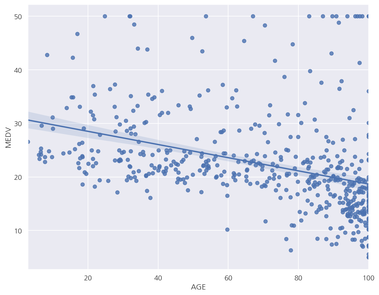
- AGE와 MEDV의 산점도를 보면 음의 상관관계가 있어 보인다.
부분회귀 플롯
statsmodels.api 패키지에 graphics.plot_partregress()로 부분회귀 플롯을 그릴 수 있다.
함수에 대한 설명은 다음과 같다.
plot_partregress(endog, exog_i, exog_others, data=None, obs_labels=True, ret_coords=False)
-
endog: 종속변수 문자열
-
exog_i: 분석 대상이 되는 독립변수 문자열
-
exog_others: 나머지 독립변수 문자열의 리스트
-
data: 모든 데이터가 있는 데이터프레임
-
obs_labels: 데이터 라벨링 여부
-
ret_coords: 잔차 데이터 반환 여부
# 나머지 독립변수 (상수항 포함)
others = list(set(df.columns).difference(set(["MEDV", "AGE"])))

plot, resids = sm.graphics.plot_partregress(
    "MEDV", "AGE", others, data=df, obs_labels=False, ret_coords=True
)

plt.show()
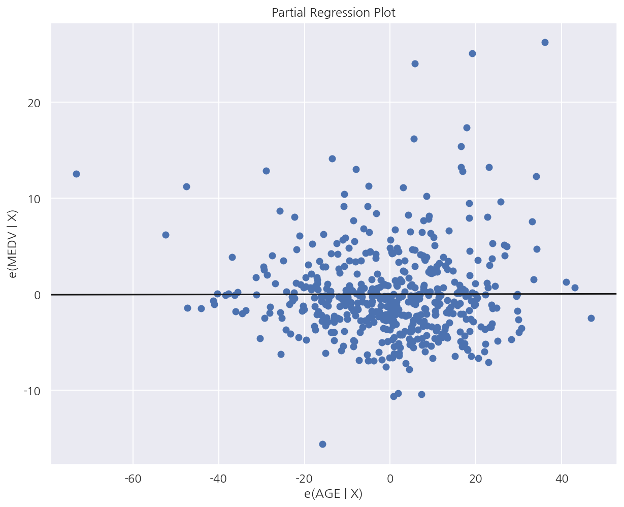
-
x축: AGE를 종속변수, 원래 종속변수인 MEDV를 제외한 나머지 변수를 독립변수로 하였을 때 잔차
-
y축: MEDV를 종속변수, AGE를 제외한 나머지 변수를 독립변수로 하였을 때 잔차
-
부분회귀 플롯으로 보았을 때 AGE와 MEDV간의 상관관계가 없음을 알 수 있다.
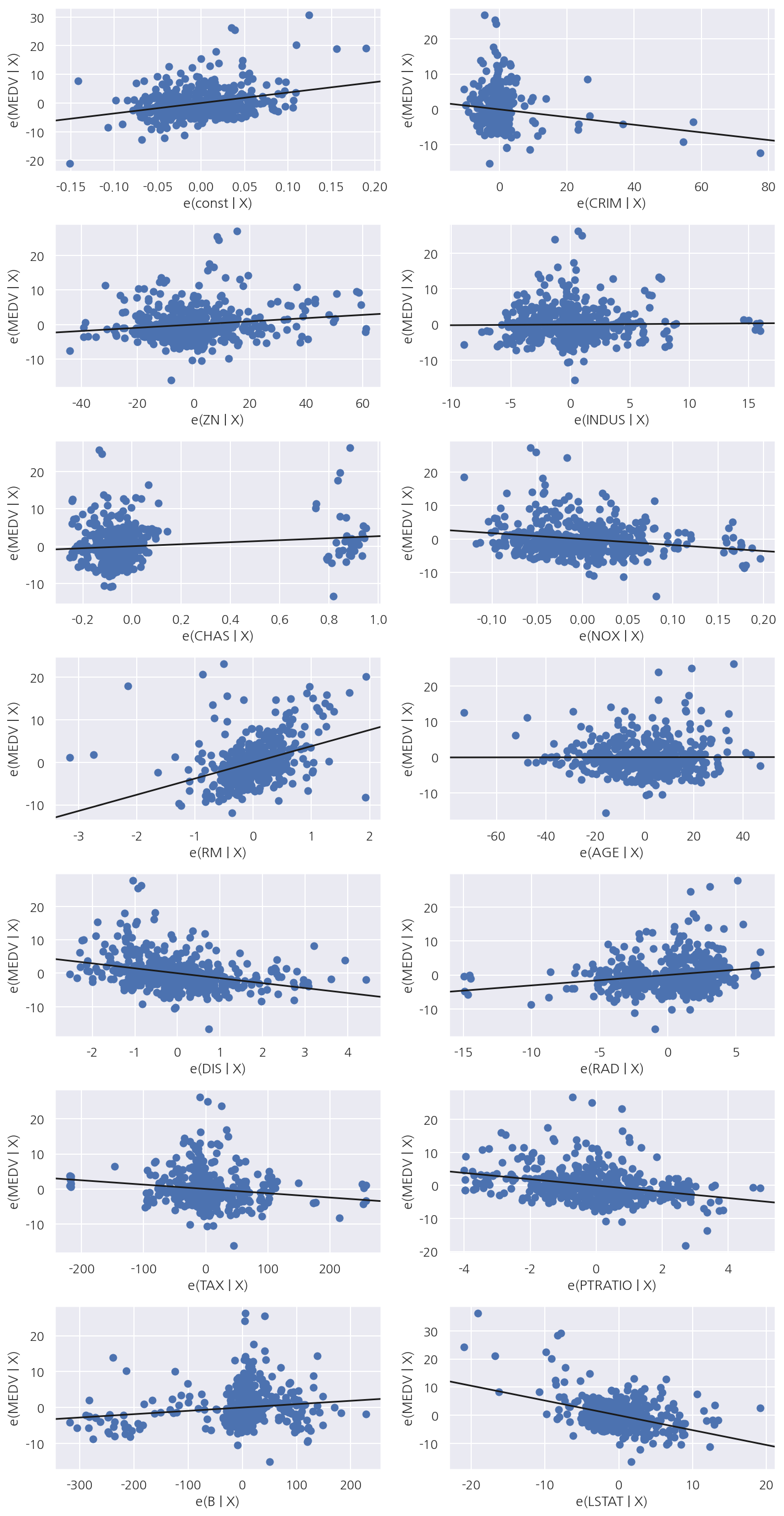
전체 부분회귀 플롯
graphics.plot_partregress_grid(result, fig)를 이용하여 모든 독립변수에 대해 부분회귀 플롯을 그릴 수 있다.
-
result: 회귀분석 결과 객체
-
fig: plt.figure 객체
fig = plt.figure(figsize=(10, 20))
sm.graphics.plot_partregress_grid(result_boston, fig=fig)
fig.suptitle("")
plt.show()
4.5.2 CCPR
CCPR(Component-Component plus Residual)
CCPR 역시 부분회귀 플롯처럼 특정한 하나의 변수의 영향을 확인하는 방법이다.
-
x축은 특정한 독립변수: $x_{s}$로 사용한다.
-
y축은 전체 독립변수를 사용한 회귀분석시 잔차에서 $\beta_{s}x_{s}$를 더해준 값을 사용한다.
-
즉, $x_{s}$와 $x_{s}$의 영향을 제외한 잔차의 산점도이다.
statsmodels.api 패키지에 graphics.plot_ccpr()로 CCPR을 그릴 수 있다.
함수에 대한 설명은 다음과 같다.
graphics.plot_ccpr(result, exog_idx)
-
result: 회귀분석 결과 객체
-
exog_idx: 분석 대상이 되는 독립변수 문자열
sm.graphics.plot_ccpr(result_boston, "AGE")

plt.show()
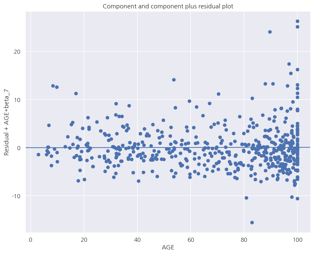
-
x축: AGE
-
y축: 기존 회귀적합모형의 잔차 + $\hat{\beta}AGE$
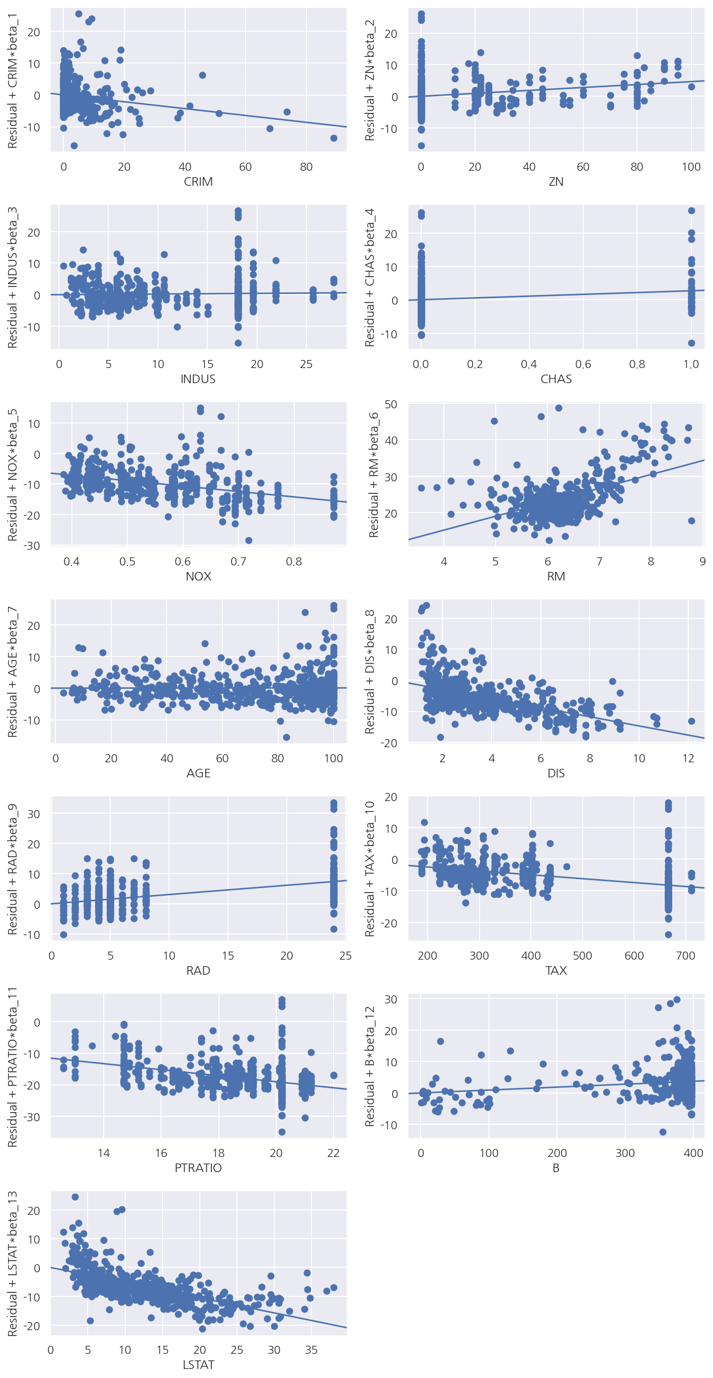
전체 CCPR
graphics.plot_ccpr_grid(result, fig)
-
result: 회귀분석 결과 객체
-
fig: plt.figure 객체
fig = plt.figure(figsize=(10, 20))

sm.graphics.plot_ccpr_grid(result_boston, fig=fig)
fig.suptitle("")

plt.show()
부분회귀 플롯 + CCPR
graphics.plot_regress_exog(result, exog_idx)
-
result: 회귀분석 결과 객체
-
exog_idx: 분석 대상이 되는 독립변수 문자열
sm.graphics.plot_regress_exog(result_boston, "AGE")

plt.show()
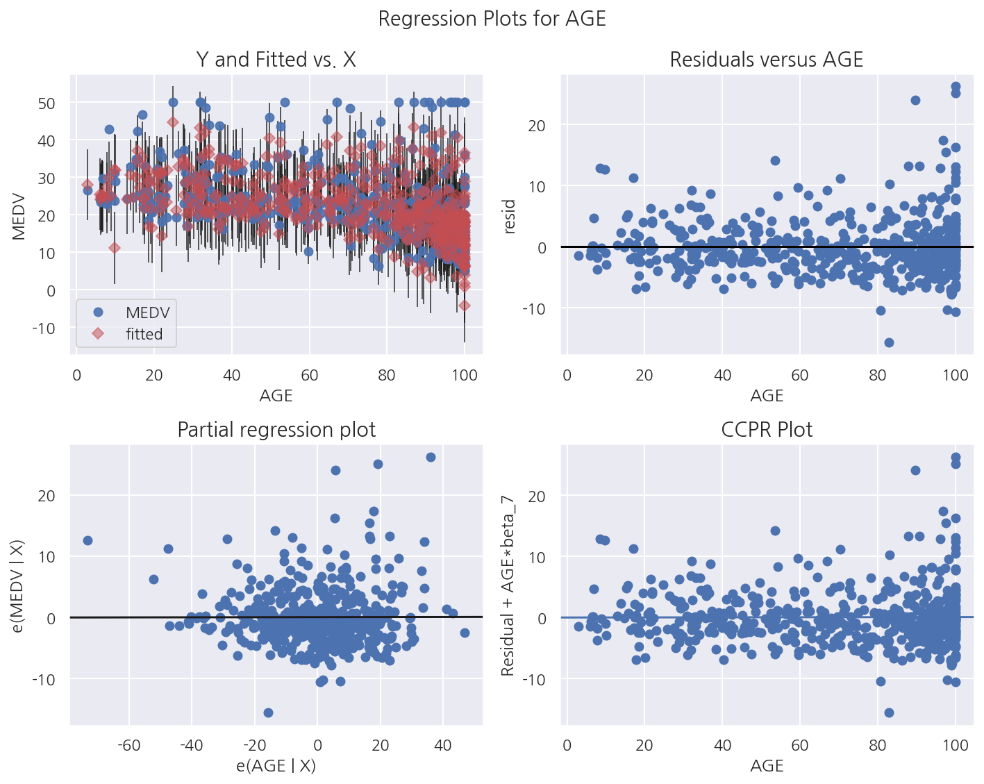
- 부분회귀 플롯과 CCPR뿐 아니라 산점도(예측값 포함), 잔차도를 함께 그려준다.
Leave a comment