
[Python] 데이터 사이언스 스쿨 - 4.2 선형 회귀분석의 기초
Updated:
데이터 사이언스 스쿨 자료를 토대로 공부한 내용입니다.
실습과정에서 필요에 따라 내용의 누락 및 추가, 수정사항이 있습니다.
기본 세팅
import numpy as np
import pandas as pd

import matplotlib as mpl
import matplotlib.pyplot as plt
import seaborn as sns

import warnings
%matplotlib inline
%config InlineBackend.figure_format = 'retina'

mpl.rc('font', family='NanumGothic') # 폰트 설정
mpl.rc('axes', unicode_minus=False) # 유니코드에서 음수 부호 설정

# 차트 스타일 설정
sns.set(font="NanumGothic", rc={"axes.unicode_minus":False}, style='darkgrid')
plt.rc("figure", figsize=(10,8))

warnings.filterwarnings("ignore")
4.2 선형 회귀분석의 기초
$n$개의 관측값을 가지는 $i$번째 독립변수 $x_i$는 다음과 같이 벡터로 표현가능하다. [$n$ x $1$]
\[x_i = \begin{bmatrix} x_{i1} \\ x_{i2} \\ \vdots \\ x_{in} \end{bmatrix}\]$n$개의 관측값을 가지고 $k-1$개의 독립변수를 가지는 행렬 $X$는 다음과 같다. [절편 포함: $n$ x $k$]
\[X = \begin{bmatrix} 1 & x_1 & x_2 & \cdots & x_p \end{bmatrix} \ = \begin{bmatrix} 1 & x_{11} & x_{21} & \cdots & x_{(k-1)1} \\ 1 & x_{12} & x_{22} & \cdots & x_{(k-1)2} \\ \vdots & \vdots & \vdots & \vdots & \vdots \\ 1 & x_{1n} & x_{2n} & \cdots & x_{(k-1)n} \\ \end{bmatrix}\]회귀계수 $\beta$ [$k$ x 1], 오차 $\epsilon$ [$n$ x 1], 종속변수 $Y$ [$n$ x 1]는 다음과 같다.
\[\beta = \begin{bmatrix} \beta_{0} \\ \beta_{1} \\ \vdots \\ \beta_{p} \end{bmatrix} , \quad \epsilon = \begin{bmatrix} \epsilon_{0} \\ \epsilon_{1} \\ \vdots \\ \epsilon_{n} \end{bmatrix} , \quad Y = \begin{bmatrix} y_{0} \\ y_{1} \\ \vdots \\ y_{n} \end{bmatrix} = X\beta + \epsilon\]-
만약 $X^{T}X$ 행렬의 역행렬이 존재한다면 추정회귀계수 $\hat{\beta}$ 은 다음과 같다.
-
$\hat{\beta} = (X^{T}X)^{-1}X^{T}Y$
-
$X^{T}X$ 행렬의 역행렬이 존재하기 위해선 각 독립변수가 서로 독립이어야 한다.
4.2.1 Numpy를 이용한 선형 회귀분석
from sklearn.datasets import make_regression
import statsmodels.api as sm

# n=200, p=1, epsilon~N(0,10)
X0, Y, B = make_regression(
    n_samples=200, n_features=1, bias=100, noise=10, coef=True, random_state=1
)

X = sm.add_constant(X0) # 상수항 결합
Y = Y.reshape(len(Y), 1)

# 모회귀계수
print("회귀계수 베타0:", 100)
print("회귀계수 베타1:", B.round(3))
print("-" * 30)

# 추정회귀계수
B_hat = np.linalg.inv(X.T @ X) @ X.T @ Y

print("추정회귀계수 베타0:", B_hat[0,0].round(3))
print("추정회귀계수 베타1:", B_hat[1,0].round(3))
회귀계수 베타0: 100
회귀계수 베타1: 86.448
------------------------------
추정회귀계수 베타0: 99.792
추정회귀계수 베타1: 86.962
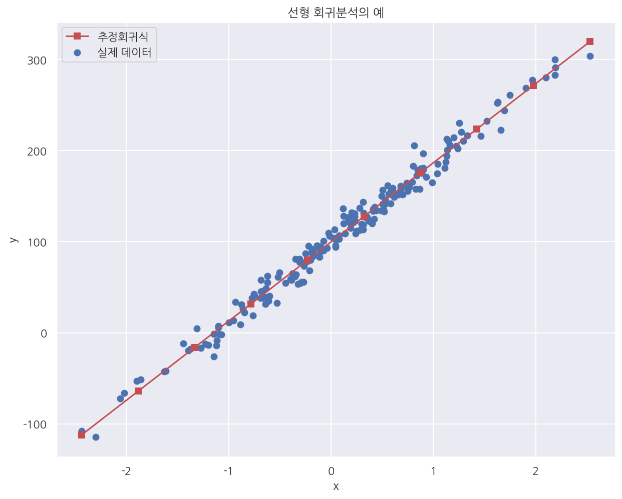
- 실제 회귀계수와 비슷한 값으로 추정한 것을 확인 할 수 있다.
# 그래프로 확인하기
x_new = np.linspace(np.min(X), np.max(X), 10)
X_new = sm.add_constant(x_new)
y_pred = np.dot(X_new, B_hat) # 예측값

plt.figure(figsize= (10,8))

plt.scatter(X0, Y, label="실제 데이터")
plt.plot(x_new, y_pred, 'rs-', label="추정회귀식")

plt.xlabel("x")
plt.ylabel("y")
plt.title("선형 회귀분석의 예")
plt.legend()

plt.show()
4.2.2 scikit-learn 패키지를 사용한 선형 회귀분석
from sklearn.linear_model import LinearRegression

model = LinearRegression(fit_intercept=True).fit(X0,Y)

print("추정회귀계수 베타0:", model.intercept_[0].round(3))
print("추정회귀계수 베타1:", model.coef_[0][0].round(3))
추정회귀계수 베타0: 99.792
추정회귀계수 베타1: 86.962
-
LinearRegression()을 이용해 넘파이에서 수기로 계산한 값과 같은 결과를 얻었다. -
디폴트로 절편을 생성하고 절편계수, 회귀계수는 각각 intercept_, coef_ 속성으로 확인 가능하다.
model.predict([[-2], [-1], [0], [1], [2]])
array([[-74.13191534],
       [ 12.82979668],
       [ 99.79150869],
       [186.7532207 ],
       [273.71493272]])
-
predict()를 이용해 새로운 x값에 대해 추정값을 구할 수 있다. -
이때 x는 2차원 배열로 기입해야한다.
-
sklearn패캐지의 대부분의 모델은fit(),predict()를 이용해서 학습하고 예측한다.
4.2.3 statsmodels 패키지를 사용한 선형 회귀분석
data = pd.DataFrame({"x": X0[:, 0], "y": Y[:, 0]})
data
| x | y | |
|---|---|---|
| 0 | 0.232495 | 127.879017 |
| 1 | -0.038696 | 93.032914 |
| 2 | 0.550537 | 161.857508 |
| 3 | 0.503185 | 141.692050 |
| 4 | 2.186980 | 283.260119 |
| ... | ... | ... |
| 195 | -0.172428 | 87.874277 |
| 196 | -1.199268 | -13.626664 |
| 197 | 1.462108 | 216.106619 |
| 198 | 1.131629 | 212.743149 |
| 199 | 0.495211 | 150.017589 |
200 rows × 2 columns
독립변수와 종속변수가 다른 데이터 프레임에 존재하는 경우
# x에 상수항을 수기로 추가해주어야 한다.
dfy = data[["y"]]
dfX = sm.add_constant(data[["x"]])

model = sm.OLS(dfy, dfX)
result = model.fit()
print(result.summary())
                            OLS Regression Results
==============================================================================
Dep. Variable:                      y   R-squared:                       0.985
Model:                            OLS   Adj. R-squared:                  0.985
Method:                 Least Squares   F-statistic:                 1.278e+04
Date:                Fri, 11 Jun 2021   Prob (F-statistic):          8.17e-182
Time:                        18:26:42   Log-Likelihood:                -741.28
No. Observations:                 200   AIC:                             1487.
Df Residuals:                     198   BIC:                             1493.
Df Model:                           1
Covariance Type:            nonrobust
==============================================================================
                 coef    std err          t      P>|t|      [0.025      0.975]
------------------------------------------------------------------------------
const         99.7915      0.705    141.592      0.000      98.402     101.181
x             86.9617      0.769    113.058      0.000      85.445      88.479
==============================================================================
Omnibus:                        1.418   Durbin-Watson:                   1.690
Prob(Omnibus):                  0.492   Jarque-Bera (JB):                1.059
Skew:                           0.121   Prob(JB):                        0.589
Kurtosis:                       3.262   Cond. No.                         1.16
==============================================================================

Notes:
[1] Standard Errors assume that the covariance matrix of the errors is correctly specified.
OLS()로 같은 회귀계수가 출력되었으며summary()로 결정계수 등 다양한 정보를 확인 가능하다.
독립변수와 종속변수가 같은 데이터 프레임에 존재하는 경우
model = sm.OLS.from_formula("y ~ x", data = data)
result = model.fit()
print(result.summary())
                            OLS Regression Results
==============================================================================
Dep. Variable:                      y   R-squared:                       0.985
Model:                            OLS   Adj. R-squared:                  0.985
Method:                 Least Squares   F-statistic:                 1.278e+04
Date:                Fri, 11 Jun 2021   Prob (F-statistic):          8.17e-182
Time:                        18:26:42   Log-Likelihood:                -741.28
No. Observations:                 200   AIC:                             1487.
Df Residuals:                     198   BIC:                             1493.
Df Model:                           1
Covariance Type:            nonrobust
==============================================================================
                 coef    std err          t      P>|t|      [0.025      0.975]
------------------------------------------------------------------------------
Intercept     99.7915      0.705    141.592      0.000      98.402     101.181
x             86.9617      0.769    113.058      0.000      85.445      88.479
==============================================================================
Omnibus:                        1.418   Durbin-Watson:                   1.690
Prob(Omnibus):                  0.492   Jarque-Bera (JB):                1.059
Skew:                           0.121   Prob(JB):                        0.589
Kurtosis:                       3.262   Cond. No.                         1.16
==============================================================================

Notes:
[1] Standard Errors assume that the covariance matrix of the errors is correctly specified.
-
독립변수 종속변수가 같은 데이터 프레임에 존재하는 경우
OLS.from_formula()로 직접 식을 적어준다. -
회귀계수는 같은 값으로 출력된 것을 확인 가능하다.
result.predict({"x": [-2, -1, 0, 1, 2] })
0    -74.131915
1     12.829797
2     99.791509
3    186.753221
4    273.714933
dtype: float64
-
LinearRegression()처럼predict()를 이용해 새로운 x값에 대한 추정값을 구할 수 있다. -
predict()외의params,resid등 다양한 속성, 메소드가 내장되어 있다.
Leave a comment