
[Python] 모두의 딥러닝 - 04. 딥러닝 기본기 다지기[데이터 다루기]
Updated:
모두의 딥러닝 교재를 토대로 공부한 내용입니다.
실습과정에서 필요에 따라 코드나 이론에 대한 추가, 수정사항이 있습니다.
기본 세팅
import numpy as np
import pandas as pd

import matplotlib as mpl
import matplotlib.pyplot as plt
import seaborn as sns

import warnings
%matplotlib inline
%config InlineBackend.figure_format = 'retina'

mpl.rc('font', family='NanumGothic') # 폰트 설정
mpl.rc('axes', unicode_minus=False) # 유니코드에서 음수 부호 설정

# 차트 스타일 설정
sns.set(font="NanumGothic", rc={"axes.unicode_minus":False}, style='darkgrid')
plt.rc("figure", figsize=(10,8))

warnings.filterwarnings("ignore")
11. 데이터 다루기
이번 챕터에서는 피마 인디언 데이터를 이용해서 딥러닝 모델을 실행해볼 것이다.
참고로 머신러닝 완벽가이드에서 피마 인디언 데이터로 로지스틱 회귀 성능 평가를 했었다.
11.1 데이터 조사
먼저 사용할 데이터의 구조는 다음과 같다.
-
pregnant: 과거 임신 횟수
-
plasma: 포도당 부하 검사 2시간 후 공복 혈당 농도
-
pressure: 확장기 혈압
-
thickness: 삼두근 피부 주름 두께
-
insulin: 혈청 인슐린
-
BMI: 체질량 지수
-
pedigree: 당뇨병 가족력
-
age: 나이
-
class: 당뇨 여부 (타겟)
# 데이터 불러오기
df = pd.read_csv("deeplearning/dataset/pima-indians-diabetes.csv",
                names = ["pregnant", "plasma", "pressure", "thickness",
                         "insulin", "BMI", "pedigree", "age", "class"])
df.head()
| pregnant | plasma | pressure | thickness | insulin | BMI | pedigree | age | class | |
|---|---|---|---|---|---|---|---|---|---|
| 0 | 6 | 148 | 72 | 35 | 0 | 33.6 | 0.627 | 50 | 1 |
| 1 | 1 | 85 | 66 | 29 | 0 | 26.6 | 0.351 | 31 | 0 |
| 2 | 8 | 183 | 64 | 0 | 0 | 23.3 | 0.672 | 32 | 1 |
| 3 | 1 | 89 | 66 | 23 | 94 | 28.1 | 0.167 | 21 | 0 |
| 4 | 0 | 137 | 40 | 35 | 168 | 43.1 | 2.288 | 33 | 1 |
- 데이터를 불러왔으며 csv 파일에 헤더 정보가 없어
names로 직접 지정하였다.
df.shape
(768, 9)
- 총 768개의 샘플로 8개의 피처, 타겟으로 구성되어 있다.
df.info()
<class 'pandas.core.frame.DataFrame'>
RangeIndex: 768 entries, 0 to 767
Data columns (total 9 columns):
 #   Column     Non-Null Count  Dtype
---  ------     --------------  -----
 0   pregnant   768 non-null    int64
 1   plasma     768 non-null    int64
 2   pressure   768 non-null    int64
 3   thickness  768 non-null    int64
 4   insulin    768 non-null    int64
 5   BMI        768 non-null    float64
 6   pedigree   768 non-null    float64
 7   age        768 non-null    int64
 8   class      768 non-null    int64
dtypes: float64(2), int64(7)
memory usage: 54.1 KB
- 결측값은 없다.
df[["pregnant", "class"]].groupby(["pregnant"], as_index=False).mean().sort_values(by="pregnant", ascending=True)
| pregnant | class | |
|---|---|---|
| 0 | 0 | 0.342342 |
| 1 | 1 | 0.214815 |
| 2 | 2 | 0.184466 |
| 3 | 3 | 0.360000 |
| 4 | 4 | 0.338235 |
| 5 | 5 | 0.368421 |
| 6 | 6 | 0.320000 |
| 7 | 7 | 0.555556 |
| 8 | 8 | 0.578947 |
| 9 | 9 | 0.642857 |
| 10 | 10 | 0.416667 |
| 11 | 11 | 0.636364 |
| 12 | 12 | 0.444444 |
| 13 | 13 | 0.500000 |
| 14 | 14 | 1.000000 |
| 15 | 15 | 1.000000 |
| 16 | 17 | 1.000000 |
-
간단하게 임신 횟수와 당뇨병 발병 확률에 대해 살펴봤다.
-
groupby()에as_index를 False로 설정하여서 바로 컬럼으로 사용 가능하다.
11.2 데이터 시각화
corr_M = df.corr()

#
sns.heatmap(corr_M,
            linewidths=0.1,
            vmax = 0.5, # 색상의 밝기 조절
            cmap = plt.cm.gist_heat,
            annot=True)

plt.show()
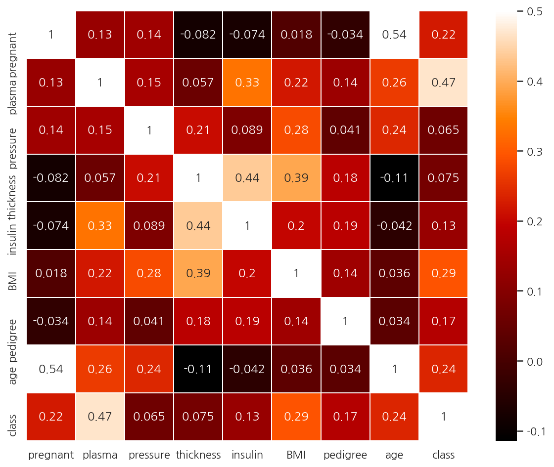
-
class와 가장 높은 상관관계를 가지는 피처는 plasma로 나타난다.
-
두 관계를 좀 더 자세히 살펴보자.
grid = sns.FacetGrid(df, col="class")
grid.map(plt.hist, "plasma", bins=10)

plt.show()
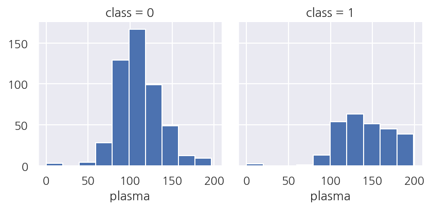
-
class가 1인 경우는 plasma가 높은 값이 많았으며 특히 150인 이상인 경우가 많다.
-
plasma가 class를 구분하는데 중요한 피처임을 알 수 있다.
-
참고로 머신러닝의 경우는 중요한 피처를 뽑는 과정도 데이터 전처리 과정에 포함하는 반면,
-
딥러닝은 중요한 피처를 내부적으로 뽑아주므로 이 과정이 필요 없다고 한다.
-
머신러닝에서도 feature_importance를 사용한 경험이 있는데 좀 더 딥러닝을 봐야 차이를 알 것 같다.
11.3 예측
import tensorflow as tf

# 시드 설정
np.random.seed(3)
tf.random.set_seed(3)

# 데이터 불러오기
dataset = np.loadtxt("deeplearning/dataset/pima-indians-diabetes.csv", delimiter = ",")
X = dataset[:,:8]
Y = dataset[:,8]
- 사실 시드 설정은 모델 실행이랑 같은 셀에 넣어두어야 하는데 따로 보려고 분리해두었다.
from tensorflow.keras.models import Sequential
from tensorflow.keras.layers import Dense

# 모델 설정
model = Sequential()
model.add(Dense(12, input_dim=8, activation="relu"))
model.add(Dense(8, activation="relu"))
model.add(Dense(1, activation="sigmoid"))
- 모델은 입력층에 모든 피처를 사용하며 2개의 은닉층을 거쳐 1개의 값을 출력하게 설정하였다.
# 모델 컴파일
model.compile(loss="binary_crossentropy",
              optimizer="adam",
              metrics=["accuracy"])
-
오차 함수는 이진 분류 문제이므로 binary_crossentropy를 사용하였다.
-
최적화 함수로는 adam을 사용하며 평가 지표는 accuracy를 사용한다.
# 모델 실행
model.fit(X, Y, epochs=10, batch_size=768)

# 결과 출력
print(f"Accuracy: {model.evaluate(X,Y, verbose=0)[1]: .4f}")
-
모델을 실행하고 평가한다.
-
evaluate()는 loss와 metrics 2개의 값을 가지고 있다. -
왜인지는 모르겠지만
evaluate()에서verbose를 설정하지 않으면 등호가 엄청나게 출력된다. -
개인 설정 문제인 듯 하다.
import tensorflow as tf
from tensorflow.keras.models import Sequential
from tensorflow.keras.layers import Dense

# 시드 설정
np.random.seed(3)
tf.random.set_seed(3)

# 데이터 불러오기
dataset = np.loadtxt("deeplearning/dataset/pima-indians-diabetes.csv", delimiter = ",")
X = dataset[:,:8]
Y = dataset[:,8]

# 모델 설정
model = Sequential()
model.add(Dense(12, input_dim=8, activation="relu"))
model.add(Dense(8, activation="relu"))
model.add(Dense(1, activation="sigmoid"))

# 모델 컴파일
model.compile(loss="binary_crossentropy",
              optimizer="adam",
              metrics=["accuracy"])

# 모델 실행
model.fit(X, Y, epochs=200, batch_size=10)

# 결과 출력
print("-"*100)
print(f"Accuracy: {model.evaluate(X,Y, verbose=0)[1]: .4f}")
Train on 768 samples
Epoch 1/200
768/768 [==============================] - 1s 880us/sample - loss: 11.4155 - accuracy: 0.6198
Epoch 2/200
768/768 [==============================] - 0s 141us/sample - loss: 6.4242 - accuracy: 0.6159
Epoch 3/200
768/768 [==============================] - 0s 123us/sample - loss: 3.6949 - accuracy: 0.5221
Epoch 4/200
768/768 [==============================] - 0s 134us/sample - loss: 2.2150 - accuracy: 0.5169
Epoch 5/200
768/768 [==============================] - 0s 144us/sample - loss: 1.3725 - accuracy: 0.5182
Epoch 6/200
768/768 [==============================] - 0s 224us/sample - loss: 0.9083 - accuracy: 0.5586
Epoch 7/200
768/768 [==============================] - 0s 160us/sample - loss: 0.7783 - accuracy: 0.5547
Epoch 8/200
768/768 [==============================] - 0s 153us/sample - loss: 0.7476 - accuracy: 0.6172 - loss: 0.7556 - accuracy: 0.61
Epoch 9/200
768/768 [==============================] - 0s 260us/sample - loss: 0.7330 - accuracy: 0.6615
Epoch 10/200
768/768 [==============================] - 0s 243us/sample - loss: 0.7014 - accuracy: 0.6602
...
Epoch 191/200
768/768 [==============================] - 0s 268us/sample - loss: 0.4975 - accuracy: 0.7266
Epoch 192/200
768/768 [==============================] - 0s 266us/sample - loss: 0.5037 - accuracy: 0.7240
Epoch 193/200
768/768 [==============================] - 0s 246us/sample - loss: 0.5086 - accuracy: 0.7240
Epoch 194/200
768/768 [==============================] - 0s 246us/sample - loss: 0.4965 - accuracy: 0.7266
Epoch 195/200
768/768 [==============================] - 0s 237us/sample - loss: 0.5009 - accuracy: 0.7201
Epoch 196/200
768/768 [==============================] - 0s 228us/sample - loss: 0.4923 - accuracy: 0.7344
Epoch 197/200
768/768 [==============================] - 0s 232us/sample - loss: 0.4904 - accuracy: 0.7253
Epoch 198/200
768/768 [==============================] - 0s 243us/sample - loss: 0.4944 - accuracy: 0.7240
Epoch 199/200
768/768 [==============================] - 0s 237us/sample - loss: 0.4935 - accuracy: 0.7214
Epoch 200/200
768/768 [==============================] - 0s 246us/sample - loss: 0.4979 - accuracy: 0.7357
----------------------------------------------------------------------------------------------------
Accuracy:  0.7253
- 약 72.53%의 정확도로 나타난다.
Leave a comment